Librosa 1.0 is finally here, after approximately 16 months of development by many (new) contributors. In this post, I’ll summarize what’s new and important with this release.

Why 1.0 now?

Librosa has been in development since 2012. We’ve aimed to produce a “major” release every year, but this has slowed down a little as the project has matured. And, to be completely transparent, I’ve had less time outside of summer to devote to development and maintenance.

Throughout our entire development history, librosa has been versioned at 0.x, but without a formal definition of what exactly that meant beyond a vague attempt at implementing semantic versioning (SemVer). Technically, SemVer allows for 0.x releases to change API without notice, though we’ve tried to be better behaved than that with proper deprecation cycles. Still, at this point, 0.x does not accurately reflect the stable state of librosa in 2026.

With 1.0, we are formally adopting Intended Effort Versioning (EffVer). This release is essentially meant to codify the 0.x series API going forward, while making it easier for us to implement deliberate API changes in the future as needed.

If you have code that worked on 0.11, it should work essentially out of the box with 1.0. The few exceptions would be expired deprecations, which are noted in the changelog.

What’s new?

Let’s talk about the new features in 1.0! While the focus of this release is on stability and maintenance, we did implement a handful of new features and usability enhancements.

Display upgrades

Most of the new functionality in 1.0 has to do with visualization. We can lump these improvements into four broad categories: wave displays, spectrogram displays, multichannel displays, and display helpers.

Waveform displays

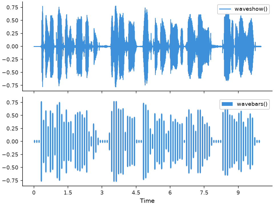
In addition to the waveshow function, we now have two additional ways to visualize waveforms.

The first, wavebars, is a simplified version of waveshow that is well suited for things like presentations or posters, where visual clarity is more important than exact fidelity to the amplitude envelope.

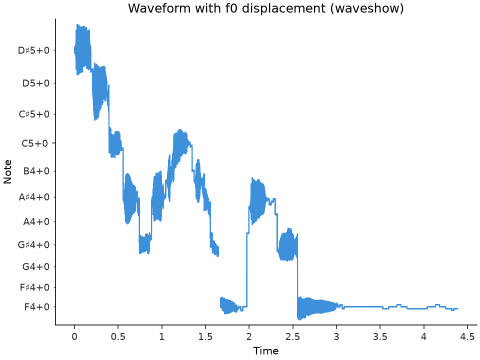
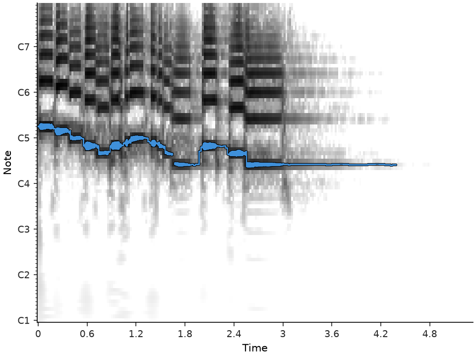
Example comparing waveshow and wavebars.

The second new function, wavef0, accepts both a signal and a fundamental frequency (f₀) sequence, and produces a frequency-displaced plot of the waveform (using either waveshow or wavebars). This can even be overlaid on top of a spectrogram display:

Example of wavef0 display.

Example of wavef0 overlaid on a spectrogram.

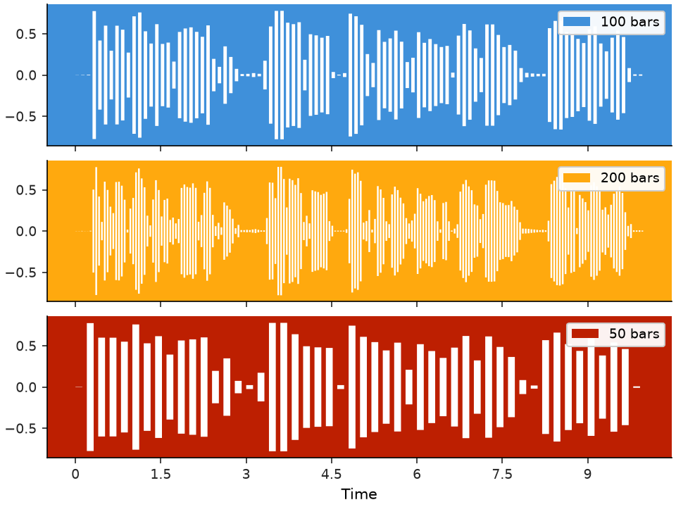
All waveform displays now additionally provide an inverted mode, where the color styling applies to the background rather than the signal. This method is commonly used in digital audio workstations to make signal displays easier to distinguish at a glance.

Example of inverted wavebars.

Spectrogram improvements

The specshow function also got some upgrades, including oct3 axis modes and balanced diverging color normalization for signed data. The biggest improvement to specshow however is the vscale parameter for controlling how value information is scaled.

In librosa 0.11 and earlier, spectrogram displays with decibel value scales required a few manual steps to prepare the data before plotting:

stft = librosa.stft(y)
stft_mag = np.abs(stft)
stft_db = librosa.amplitude_to_db(stft_mag, ref=np.max)

librosa.display.specshow(stft_db, x_axis='time', y_axis='log')

or as a one-liner,

librosa.display.specshow(librosa.amplitude_to_db(np.abs(stft), ref=np.max),
                         x_axis='time', y_axis='log')

The vscale parameter streamlines this into the following equivalent code:

stft = librosa.stft(y)

librosa.display.specshow(stft, x_axis='time', y_axis='log', vscale='dBFS')

In addition to simplifying the code that you have to write as a user, selection of a decibel vscale overrides the colormap inference to always use a sequential map. This prevents a common mistake where users provide a signed decibel value array (e.g., computed with a static reference value of 1), resulting in a diverging colormap visualization.

The vscale parameter can also be used to plot phase information and phase differential information with a cyclical colormap. The rainbowgrams example shows how to use this effectively in practice.

Multichannel displays

One of the biggest new features in 1.0 is multi-channel display. The basic architecture is to map out one of the existing display routines (e.g. waveshow or specshow) over an array of matplotlib axes, with shared parameters common to each subplot.

Where you previously could independently call waveshow on different axes for each signal, e.g.:

y_harmonic, y_percussive = librosa.effects.hpss(y)

fig, ax = plt.subplots(nrows=3, sharex=True, sharey=True)
librosa.display.waveshow(y, sr=sr, ax=ax[0], label="Original", color="C0")
librosa.display.waveshow(y_harmonic, sr=sr, ax=ax[1], label="Harmonic", color="C1")
librosa.display.waveshow(y_percussive, sr=sr, ax=ax[2], label="Percussive", color="C2")

you can now do the same in one shot:

fig, ax = plt.subplots(nrows=3, sharex=True, sharey=True)
librosa.display.multiplot("waveshow", y, y_harmonic, y_percussive,
                          sr=sr,
                          labels=["Original", "Harmonic", "Percussive"],
                          axes=ax)
fig.legend(loc="outside right")

to produce the following figure: 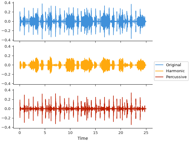Example of multiplot with waveshow.

The multichannel display tutorial goes into much more detail about all this function can do.

Helpers

Finally, we’ve added a few quality-of-life improvements to make generating plots just a little easier.

highlight makes it easy to add path effects (outlines or shadows) to matplotlib artists so they appear more visibly overlaid on spectrogram displays.
colorbar_db and colorbar_phase provide simple ways to construct colorbars with appropriate labeling for decibel- and angle-valued data, respectively.

New features

Compared to display, there are not so many new feature extraction or transformation functions in this release, but there are a few:

hybrid_tempogram combines autocorrelation- and Fourier-based tempogram representations into a single representation, which can result in a cancellation of octave errors.
metrogram summarizes the relative energy at different meters (e.g., 3/4, 4/4, 5/4) over time, which can be used to then estimate the time signature of a recording.
to_mono, to_stereo, and to_multi provide simple and flexible interfaces to mixing signals into different multi-dimensional array shapes.

Expanded tutorials

The 1.0 release coincides with an overhaul and modernization of our documentation site. A major part of this is an expansion of the tutorials section, which now includes 16 short sections to introduce specific topics, and another 13 sections with more advanced examples.

Our plan is for these sections to expand over time, and provide a more pedagogical and narrative explanation of how to use librosa effectively than the API documentation.

What’s better?

Along with new features, there have been quite a few improvements to existing functionality.

Faster import

One complaint we noticed quite often in the 0.10 and 0.11 series was that import time was becoming a substantial barrier for users. Even with lazy loading, just running import librosa was taking an unusually long amount of time before even executing any real code.

This turned out to be due to eager compilation of certain numba-optimized subroutines. When these functions were first developed, this eager compilation was necessary, but this is happily no longer the case. This is now fully resolved in librosa 1.0, and import times should be speedy again.

Stream resampling

In an earlier post on this blog, I described how to use the stream function to sequentially process a long signal instead of loading it all in bulk. One drawback noted in the previous post was that stream did not support on-the-fly sample rate conversion, and was therefore pinned to the signal’s native sampling rate. Unless you are being very careful, this can lead to some mismatch of default parameter interpretations (e.g., frame lengths) when going between load and stream-based processing.

This is no longer the case: stream now supports on the fly sample rate conversion, in exactly the same way that load does. At present, this is not enabled by default so as to preserve backward compatibility with the 0.x behavior.

Note

In the future 1.1 release, the default behavior will change to align with the default behavior of load. It’s a good idea to start making sr= an explicit parameter to stream now to avoid being surprised in the future.

Efficiency improvements

Several other functions received efficiency improvements, either in terms of speed or memory usage. One of the biggest improvements is in the viterbi function (as well as related algorithms like viterbi_discriminative and viterbi_binary). By default, the viterbi implementation now uses a sparsified transition matrix to eliminate computation of low-likelihood transitions, resulting in a substantial speedup (often 10× or more) for algorithms like pyin.

Type annotations

The type annotation coverage for the entire package has been improved several times over. While there is still some ways to go in terms of refining type annotations of numpy array return values, there is otherwise complete coverage of all functions.

What’s changing?

We should also discuss behaviors that are changing from the 0.11.0 release. There aren’t many, but they are worth noting.

Decibel scaling channel independence

amplitude_to_db and power_to_db, when provided with a function for ref parameter, will now default to operating over the trailing axes instead of the entire array. This doesn’t change behavior on single-channel data, but is necessary for multi-channel data to preserve channel independence. In 0.11 and earlier, the following code would produce different results:


# Assume stft_mag is a (2, n_freq, n_frames) array of stereo STFT magnitudes

db_left = librosa.amplitude_to_db(stft_mag[0], ref=np.max)
db_right = librosa.amplitude_to_db(stft_mag[1], ref=np.max)
db_stereo = librosa.amplitude_to_db(stft_mag, ref=np.max)
# db_stereo[0] != db_left  in 0.11
# db_stereo[1] != db_right in 0.11

While in 1.0, the results are now consistent (db_stereo[0] == db_left and db_stereo[1] == db_right).

This also affects functions which rely on decibel scaling, such as MFCC calculation.

If you need to preserve equivalency to results computed in 0.11, you can set axes=None to force ref to operate over all axes:

librosa.amplitude_to_db(stft_mag, ref=np.max, axes=None)  # equivalent to 0.11 behavior

Sparse arrays and matrices

A few functions in librosa rely on sparse representations, or at least provide the option to use them. Historically we have relied on scipy sparse matrices. In the 1.0 release, we are transitioning to the newer sparse array representation. This means that functions which previously returned scipy.sparse.spmatrix objects will now return scipy.sparse.sparse_array objects.

Deprecations

A few previously deprecated functions and features have been removed in 1.0, including:

audioread backend for loading audio files
The filename argument in librosa.stream (in favor of path)
The res_type argument in librosa.vqt
set_fftlib and get_fftlib
The win_length parameter in yin and pyin
The x_axis parameter in waveshow (in favor of axis)
filters.constant_q and filters.constant_q_lengths (in favor of wavelet and wavelet_lengths)

We also have a few new deprecations which will be removed in future releases:

librosa.display.cmap is being renamed to librosa.display.infer_cmap
librosa.phase_vocoder will no longer accept hop_length and n_fft parameters
random_state parameters are being replaced with rng parameters (see below).

SPEC endorsements

Another focus of the 1.0 release is to bring the package up to modern best practices in the Scientific Python community. To this end, we are now endorsing several Scientific Python Ecosystem Coordination recommendations:

SPEC0 - Minimum supported dependencies

SPEC0 recommends a time-based, rather than functionality-based policy for dropping dependencies. This will allow us to reduce the rate of incurring technical debt going forward, and maintain a healthier pace of development.

Specifically, SPEC0 states:

Support for Python versions be dropped 3 years after their initial release.

Support for core package dependencies be dropped 2 years after their initial release.

For our purposes, this means that librosa now requires the following:

Python >= 3.12
numba >= 0.61.0
numpy >= 2.1.0
scipy >= 1.15.0
scikit-learn >= 1.6.0
joblib >= 1.2
decorator >= 5.2.1
soundfile >= 0.12.1
pooch >= 1.7
soxr >= 1.0.0
lazy_loader >= 0.3
msgpack >= 1.0.5

SPEC1 - Lazy loading

SPEC1 recommends importing submodules on an as-needed basis. Librosa has supported this since 0.10.

SPEC7 - Seeding PRNGs

SPEC7 defines a standardized interface for seeding pseudo-random number generators, namely rng=. In librosa 1.0, all use of PRNGs has been migrated to this interface, with older random_state or seed parameters remaining as deprecation shims to be fully removed in the future.

What’s next?

With librosa 1.0 done, we will begin focusing on development of new features and expansion of functionality. There are already a few well-specified milestones mapped out, and we (I) would be happy to have more contributors get involved with future development. See the contributing guide for more information on how to get involved.

Acknowledgments

Thanks to all contributors to the 1.0 release, including (but not limited to) the following in no specific order: Suhas Holla Karkada Chandrashekar, Gopesh Pandey, Daniel Fernandes, Kayvan Zahiri, Ethan Cajetan Menezes, Valerian Coelho, Imrul Huda, ejwong, AD, Daniel Haas B, Joren Hammudoglu, Cameron Brooks, Petra Kuhnle, cookesan, Haydn Lam, Fadel Akram, emilazy, Ale Lloveras, Stefan Balke, and Vincent Lostanlen.