Caution

You're reading the documentation for a development version. For the latest released version, please have a look at 0.9.1.

librosa.util.cyclic_gradient

librosa.util.cyclic_gradient(data, *, edge_order=1, axis=- 1)

Estimate the gradient of a function over a uniformly sampled, periodic domain.

This is essentially the same as np.gradient, except that edge effects are handled by wrapping the observations (i.e. assuming periodicity) rather than extrapolation.

Parameters

datanp.ndarray

The function values observed at uniformly spaced positions on a periodic domain

edge_order{1, 2}

The order of the difference approximation used for estimating the gradient

axisint

The axis along which gradients are calculated.

Returns

gradnp.ndarray like data

The gradient of data taken along the specified axis.

See also

numpy.gradient

Examples

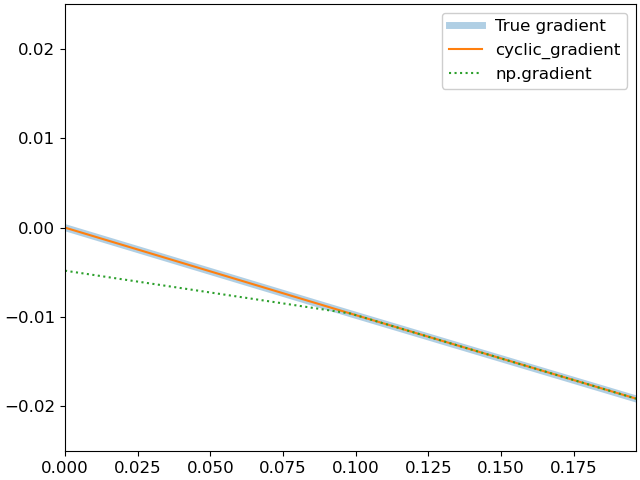
This example estimates the gradient of cosine (-sine) from 64 samples using direct (aperiodic) and periodic gradient calculation.

>>> import matplotlib.pyplot as plt
>>> x = 2 * np.pi * np.linspace(0, 1, num=64, endpoint=False)
>>> y = np.cos(x)
>>> grad = np.gradient(y)
>>> cyclic_grad = librosa.util.cyclic_gradient(y)
>>> true_grad = -np.sin(x) * 2 * np.pi / len(x)
>>> fig, ax = plt.subplots()
>>> ax.plot(x, true_grad, label='True gradient', linewidth=5,
...          alpha=0.35)
>>> ax.plot(x, cyclic_grad, label='cyclic_gradient')
>>> ax.plot(x, grad, label='np.gradient', linestyle=':')
>>> ax.legend()
>>> # Zoom into the first part of the sequence
>>> ax.set(xlim=[0, np.pi/16], ylim=[-0.025, 0.025])