Caution

You're reading an old version of this documentation. If you want up-to-date information, please have a look at 0.10.1.

librosa.lpc

librosa.lpc(y, order)

Linear Prediction Coefficients via Burg’s method

This function applies Burg’s method to estimate coefficients of a linear filter on y of order order. Burg’s method is an extension to the Yule-Walker approach, which are both sometimes referred to as LPC parameter estimation by autocorrelation.

It follows the description and implementation approach described in the introduction by Marple. [1] N.B. This paper describes a different method, which is not implemented here, but has been chosen for its clear explanation of Burg’s technique in its introduction.

[1]

Larry Marple. A New Autoregressive Spectrum Analysis Algorithm. IEEE Transactions on Accoustics, Speech, and Signal Processing vol 28, no. 4, 1980.

Parameters:

ynp.ndarray

Time series to fit

orderint > 0

Order of the linear filter

Returns:

anp.ndarray of length order + 1

LP prediction error coefficients, i.e. filter denominator polynomial

Raises:

ParameterError

• If y is not valid audio as per librosa.util.valid_audio

• If order < 1 or not integer

FloatingPointError

• If y is ill-conditioned

See also

scipy.signal.lfilter

Examples

Compute LP coefficients of y at order 16 on entire series

>>> y, sr = librosa.load(librosa.ex('trumpet'))
>>> librosa.lpc(y, 16)

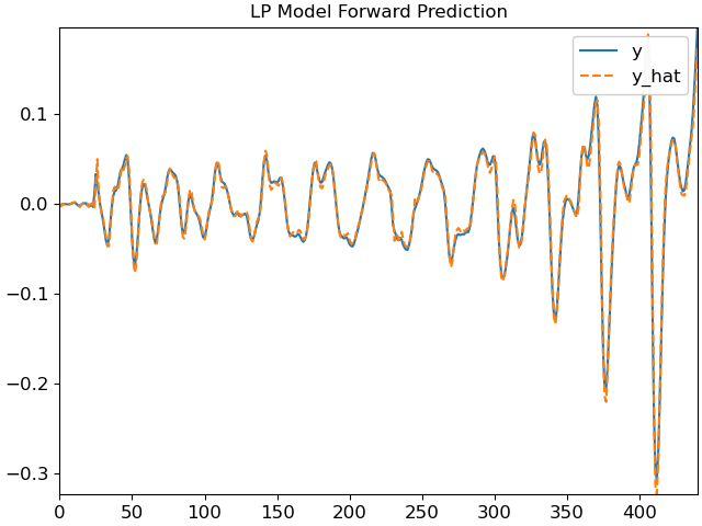
Compute LP coefficients, and plot LP estimate of original series

>>> import matplotlib.pyplot as plt
>>> import scipy
>>> y, sr = librosa.load(librosa.ex('trumpet'), duration=0.020)
>>> a = librosa.lpc(y, 2)
>>> b = np.hstack([[0], -1 * a[1:]])
>>> y_hat = scipy.signal.lfilter(b, [1], y)
>>> fig, ax = plt.subplots()
>>> ax.plot(y)
>>> ax.plot(y_hat, linestyle='--')
>>> ax.legend(['y', 'y_hat'])
>>> ax.set_title('LP Model Forward Prediction')