Caution
You're reading the documentation for a development version. For the latest released version, please have a look at 0.11.0.
librosa.display.specshow
- librosa.display.specshow(data, *, x_coords=None, y_coords=None, x_axis=None, y_axis=None, vscale=None, sr=22050, hop_length=512, n_fft=None, win_length=None, fmin=None, fmax=None, tempo_min=16, tempo_max=480, tuning=0.0, bins_per_octave=12, key='C:maj', Sa=None, mela=None, thaat=None, auto_aspect=True, htk=False, unicode=True, intervals=None, unison=None, top_db=80.0, cmap_seq='magma', cmap_bool='gray_r', cmap_div='coolwarm', cmap_cyclic='twilight_shifted', div_thresh=0.0, ax=None, **kwargs)[source]
Display a spectrogram/chromagram/cqt/etc.
For a detailed overview of this function, see Using display.specshow
- Parameters:
- datanp.ndarray [shape=(d, n)]
Matrix to display (e.g., spectrogram)
- x_coords, y_coordsnp.ndarray [shape=data.shape[0 or 1]]
Optional positioning coordinates of the input data. These can be use to explicitly set the location of each element
data[i, j], e.g., for displaying beat-synchronous features in natural time coordinates.If not provided, they are inferred from
x_axisandy_axis.- x_axis, y_axisNone or str
Range for the x- and y-axes.
Valid types are:
None, ‘none’, or ‘off’ : no axis decoration is displayed.
Frequency types:
‘linear’, ‘fft’, ‘hz’ : frequency range is determined by the FFT window and sampling rate.
‘log’ : the spectrum is displayed on a log scale.
‘oct3’ : the spectrum is displayed on a log scale with frequencies marked in scientific notation at 1/3-octave intervals
‘fft_note’: the spectrum is displayed on a log scale with pitches marked.
‘fft_svara’: the spectrum is displayed on a log scale with svara marked.
‘mel’ : frequencies are determined by the mel scale.
‘mel_oct3’ : like ‘oct3’ above, but using the mel scale.
‘cqt_hz’ : frequencies are determined by the CQT scale.
‘cqt_oct3’ : like ‘oct3’ above, but using the CQT scale.
‘cqt_note’ : pitches are determined by the CQT scale.
‘cqt_svara’ : like cqt_note but using Hindustani or Carnatic svara
‘vqt_hz’ : like cqt_hz but using Variable-Q Transform (VQT) scale.
‘vqt_oct3’ : like ‘oct3’ above, but using the VQT scale.
‘vqt_fjs’ : like cqt_note but using Functional Just System (FJS) notation. This requires a just intonation-based variable-Q transform representation.
‘vqt_note’ : like ‘cqt_note’ but using the VQT scale.
All frequency types are plotted in units of Hz.
oct3-type use SI prefixes for frequencies, e.g., 1 kHz, 2 MHz, and are well adapted for scientific applications using high-frequency data.
Note
The ‘log’, ‘fft_note’, ‘fft_svara’, ‘log_oct3’, ‘mel’, and ‘mel_oct3’ axes use symmetric-log scaling to retain frequency bins near 0 Hz. CQT and VQT axes use logarithmic scaling.
Any spectrogram parameters (hop_length, sr, bins_per_octave, etc.) used to generate the input data should also be provided when calling
specshow.Categorical types:
‘chroma’ : pitches are determined by the chroma filters. Pitch classes are arranged at integer locations (0-11) according to a given key.
chroma_h, chroma_c: pitches are determined by chroma filters, and labeled as svara in the Hindustani (chroma_h) or Carnatic (chroma_c) according to a given thaat (Hindustani) or melakarta raga (Carnatic).
‘chroma_fjs’: pitches are determined by chroma filters using just intonation. All pitch classes are annotated.
‘tonnetz’ : axes are labeled by Tonnetz dimensions (0-5)
‘frames’ : markers are shown as frame counts.
Time types:
- ‘time’markers are shown as milliseconds, seconds, minutes, or hours.
Values are plotted in units of seconds.
‘h’ : markers are shown as hours, minutes, and seconds.
‘m’ : markers are shown as minutes and seconds.
‘s’ : markers are shown as seconds.
‘ms’ : markers are shown as milliseconds.
‘lag’ : like time, but past the halfway point counts as negative values.
‘lag_h’ : same as lag, but in hours, minutes and seconds.
‘lag_m’ : same as lag, but in minutes and seconds.
‘lag_s’ : same as lag, but in seconds.
‘lag_ms’ : same as lag, but in milliseconds.
Rhythm:
- ‘tempo’markers are shown as beats-per-minute (BPM)
using a logarithmic scale. This is useful for visualizing the outputs of feature.tempogram.
- ‘fourier_tempo’same as ‘tempo’, but used when
tempograms are calculated in the Frequency domain using feature.fourier_tempogram.
- vscalestr
Optional value transformation for data. The following are supported:
‘dB’ : decibels with 1 as a reference amplitude
‘dB[<value>]’ : decibels with the given value as a reference amplitude, e.g. ‘dB[0.1]’.
‘dB[power]’ : like above, but treating data as power rather than amplitude measurements.
‘dB[power,<value>]’ : like above, but with an explicit reference power value, e.g. ‘dB[power,0.1]’.
‘dBFS’ : decibels relative to full scale, using np.max(data) as a reference amplitude
‘dBFS[power]’ : like above, but treating data as power rather than amplitude measurements.
‘phase’ : phase values in radians, with a range of [-π, π].
‘dphase’ : unwrapped phase differences in radians. Each pixel corresponds to the residual between the observed phase and the expected phase if the frequency was stationary at the previous time step. Values are in the range of [-π, π].
‘dphase_t’ : as above, but differences are computed along the vertical axis instead of horizontal. This is intended for use with transposed spectrograms where the time axis is vertical and the frequency axis is horizontal.
Note
When using phase difference modes (dphase or dphase_t), the x and y coordinates must be provided via either the x_axis and y_axis parameters (e.g., ‘time’, ‘fft’), or explicitly by the x_coords and y_coords parameters. All time-like and frequency-like axes are supported.
- srnumber > 0 [scalar]
Sample rate used to determine time scale in x-axis.
- hop_lengthint > 0 [scalar]
Hop length, also used to determine time scale in x-axis
- n_fftint > 0 or None
Number of samples per frame in STFT/spectrogram displays. By default, this will be inferred from the shape of
dataas2 * (d - 1). Ifdatawas generated using an odd frame length, the correct value can be specified here.- win_lengthint > 0 or None
The number of samples per window. By default, this will be inferred to match
n_fft. This is primarily useful for specifying odd window lengths in Fourier tempogram displays.- fminfloat > 0 [scalar] or None
Frequency of the lowest spectrogram bin. Used for Mel, CQT, and VQT scales.
If
y_axisis cqt_hz or cqt_note andfminis not given, it is set by default tonote_to_hz('C1').- fmaxfloat > 0 [scalar] or None
Used for setting the Mel frequency scales
- tempo_minfloat > 0 [scalar]
Lowest tempo (in beats per minute) for tempogram display.
- tempo_maxfloat > 0 [scalar]
Highest tempo (in beats per minute) for tempogram display.
- tuningfloat
Tuning deviation from A440, in fractions of a bin.
This is used for CQT frequency scales, so that
fminis adjusted tofmin * 2**(tuning / bins_per_octave).- bins_per_octaveint > 0 [scalar]
Number of bins per octave. Used for CQT frequency scale.
- keystr
The reference key to use when using note axes (cqt_note, chroma).
- Safloat or int
If using Hindustani or Carnatic svara axis decorations, specify Sa.
For cqt_svara,
Sashould be specified as a frequency in Hz.For chroma_c or chroma_h,
Sashould correspond to the position of Sa within the chromagram. If not provided, Sa will default to 0 (equivalent to C)- melastr or int, optional
If using chroma_c or cqt_svara display mode, specify the melakarta raga.
- thaatstr, optional
If using chroma_h display mode, specify the parent thaat.
- auto_aspectbool
Axes will have ‘equal’ aspect if the horizontal and vertical dimensions cover the same extent and their types match.
To override, set to False.
- htkbool
If plotting on a mel frequency axis, specify which version of the mel scale to use.
False: use Slaney formula (default)
True: use HTK formula
See
core.mel_frequenciesfor more information.- unicodebool
If using note or svara decorations, setting unicode=True will use unicode glyphs for accidentals and octave encoding.
Setting unicode=False will use ASCII glyphs. This can be helpful if your font does not support musical notation symbols.
- intervalsstr or array of floats in [1, 2), optional
If using an FJS notation (chroma_fjs, vqt_fjs), the interval specification.
See
core.interval_frequenciesfor a description of supported values.- unisonstr, optional
If using an FJS notation (chroma_fjs, vqt_fjs), the pitch name of the unison interval. If not provided, it will be inferred from fmin (for VQT display) or assumed as ‘C’ (for chroma display).
- top_dbfloat
If using a decibel scale, how many dB below the peak to allow before clipping.
- cmap_seqstr or matplotlib.colors.Colormap
The name of the sequential colormap to use for decibel scales. Default is ‘magma’.
- cmap_boolstr or matplotlib.colors.Colormap
The name of the colormap to use for boolean data. Default is ‘gray_r’.
- cmap_divstr or matplotlib.colors.Colormap
The name of the diverging colormap to use for diverging data. Default is ‘coolwarm’.
- cmap_cyclicstr or matplotlib.colors.Colormap
The name of the cyclic colormap to use for phase data. Default is ‘twilight_shifted’.
- div_threshfloat
The threshold for determining whether to use a diverging colormap. If the data has values both above and below this threshold, then a diverging colormap is used.
- axmatplotlib.axes.Axes or None
Axes to plot on instead of the default plt.gca().
- **kwargsadditional keyword arguments
Arguments passed through to
matplotlib.pyplot.pcolormesh.By default, the following options are set:
rasterized=Trueshading='auto'edgecolors='None'
- Returns:
- colormesh
matplotlib.collections.QuadMesh The color mesh object produced by
matplotlib.pyplot.pcolormesh
- colormesh
See also
colorbar_dbcolorbar_phaseinfer_cmapAutomatic colormap detection
matplotlib.pyplot.pcolormesh
Notes
The
cmapoption if not provided via kwargs, is inferred from data automatically. If vscale is specified, the colormap will be sequential for decibels, and cyclic for phase and phase differences.If a diverging colormap is inferred, the color scale is normalized so that the center value (
div_thresh=0by default) is at the center of the colormap.To use matplotlib’s default colormap, explicitly set
cmap=None.Examples
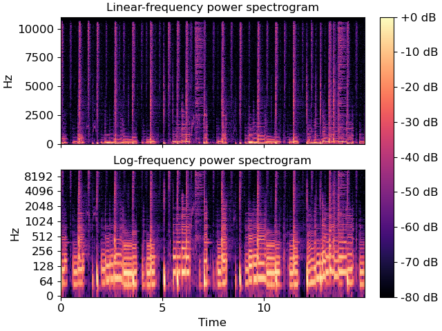
Visualize an STFT magnitude spectrum using default parameters
>>> import matplotlib.pyplot as plt
>>> y, sr = librosa.loadx('choice', duration=15)
>>> fig, ax = plt.subplots(nrows=2, ncols=1, sharex=True)
>>> D = librosa.stft(y)
>>> img = librosa.display.specshow(D, y_axis='linear', x_axis='time',
...                                vscale='dBFS', sr=sr, ax=ax[0])
>>> ax[0].set(title='Linear-frequency magnitude spectrogram')
>>> ax[0].label_outer()
Or on a logarithmic scale, and using a larger hop
>>> hop_length = 1024
>>> D = librosa.stft(y, hop_length=hop_length)
>>> librosa.display.specshow(D, y_axis='log', sr=sr, hop_length=hop_length,
...                          vscale='dBFS', x_axis='time', ax=ax[1])
>>> ax[1].set(title='Log-frequency magnitude spectrogram')
>>> ax[1].label_outer()
>>> librosa.display.colorbar_db(img, ax=ax)