Caution
You're reading the documentation for a development version. For the latest released version, please have a look at 0.11.0.
librosa.vqt
- librosa.vqt(y, *, sr=22050, hop_length=512, fmin=None, n_bins=84, intervals='equal', gamma=None, bins_per_octave=12, tuning=0.0, filter_scale=1, norm=1, sparsity=0.01, window='hann', scale=True, pad_mode='constant', res_type='soxr_hq', dtype=None)[source]
Compute the variable-Q transform of an audio signal.
This implementation is based on the recursive sub-sampling method described by [1].
- Parameters:
- ynp.ndarray [shape=(…, n)]
audio time series. Multi-channel is supported.
- srnumber > 0 [scalar]
sampling rate of
y- hop_lengthint > 0 [scalar]
number of samples between successive VQT columns.
- fminfloat > 0 [scalar]
Minimum frequency. Defaults to C1 ~= 32.70 Hz
- n_binsint > 0 or None [scalar]
Number of frequency bins, starting at
fminIf None, the number of bins will be inferred as the maximum that will fit below sr/2.- intervalsstr or array of floats in [1, 2)
Either a string specification for an interval set, e.g., ‘equal’, ‘pythagorean’, ‘ji3’, etc. or an array of intervals expressed as numbers between 1 and 2. .. see also:: librosa.interval_frequencies
- gammanumber > 0 [scalar]
Bandwidth offset for determining filter lengths.
If
gamma=0, produces the constant-Q transform.If ‘gamma=None’, gamma will be calculated such that filter bandwidths are equal to a constant fraction of the equivalent rectangular bandwidths (ERB). This is accomplished by solving for the gamma which gives:
B_k = alpha * f_k + gamma = C * ERB(f_k),
where
B_kis the bandwidth of filterkwith center frequencyf_k, alpha is the inverse of what would be the constant Q-factor, andC = alpha / 0.108is the constant fraction across all filters.Here we use
ERB(f_k) = 24.7 + 0.108 * f_k, the best-fit curve derived from experimental data in [2].- bins_per_octaveint > 0 [scalar]
Number of bins per octave
- tuningNone or float
Tuning offset in fractions of a bin.
If
None, tuning will be automatically estimated from the signal.The minimum frequency of the resulting VQT will be modified to
fmin * 2**(tuning / bins_per_octave).- filter_scalefloat > 0
Filter scale factor. Small values (<1) use shorter windows for improved time resolution.
- norm{inf, -inf, 0, float > 0}
Type of norm to use for basis function normalization. See
librosa.util.normalize.- sparsityfloat in [0, 1)
Sparsify the VQT basis by discarding up to
sparsityfraction of the energy in each basis.Set
sparsity=0to disable sparsification.- windowstr, tuple, number, or function
Window specification for the basis filters. See
filters.get_windowfor details.- scalebool
If
True, scale the VQT response by square-root the length of each channel’s filter. This is analogous tonorm='ortho'in FFT.If
False, do not scale the VQT. This is analogous tonorm=Nonein FFT.- pad_modestr
Padding mode for centered frame analysis.
See also:
librosa.stftandnumpy.pad.- res_typestr
The resampling mode for recursive downsampling.
- dtypenp.dtype
The dtype of the output array. By default, this is inferred to match the numerical precision of the input signal.
- Returns:
- VQTnp.ndarray [shape=(…, n_bins, t), dtype=np.complex]
Variable-Q value each frequency at each time.
See also
Notes
This function caches at level 20.
Examples
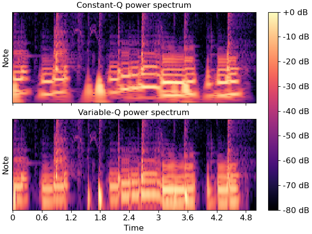
Generate and plot a variable-Q power spectrum
>>> import matplotlib.pyplot as plt
>>> y, sr = librosa.loadx('choice', duration=5)
>>> C = np.abs(librosa.cqt(y, sr=sr))
>>> V = np.abs(librosa.vqt(y, sr=sr))
>>> fig, ax = plt.subplots(nrows=2, sharex=True, sharey=True)
>>> librosa.display.specshow(C, vscale='dBFS',
...                          sr=sr, x_axis='time', y_axis='cqt_note', ax=ax[0])
>>> ax[0].set(title='Constant-Q power spectrum', xlabel=None)
>>> ax[0].label_outer()
>>> img = librosa.display.specshow(V, vscale='dBFS',
...                                sr=sr, x_axis='time', y_axis='cqt_note', ax=ax[1])
>>> ax[1].set_title('Variable-Q power spectrum')
>>> librosa.display.colorbar_db(img, ax=ax)