Caution

You're reading an old version of this documentation. If you want up-to-date information, please have a look at 0.10.2.

librosa.feature.delta

librosa.feature.delta(data, width=9, order=1, axis=-1, mode='interp', **kwargs)[source]

Compute delta features: local estimate of the derivative of the input data along the selected axis.

Delta features are computed Savitsky-Golay filtering.

Parameters:

datanp.ndarray

the input data matrix (eg, spectrogram)

widthint, positive, odd [scalar]

Number of frames over which to compute the delta features. Cannot exceed the length of data along the specified axis.

If mode='interp', then width must be at least data.shape[axis].

orderint > 0 [scalar]

the order of the difference operator. 1 for first derivative, 2 for second, etc.

axisint [scalar]

the axis along which to compute deltas. Default is -1 (columns).

modestr, {‘interp’, ‘nearest’, ‘mirror’, ‘constant’, ‘wrap’}

Padding mode for estimating differences at the boundaries.

kwargsadditional keyword arguments

See scipy.signal.savgol_filter

Returns:

delta_datanp.ndarray [shape=(d, t)]: delta matrix of data at specified order

See also

scipy.signal.savgol_filter

Notes

This function caches at level 40.

Examples

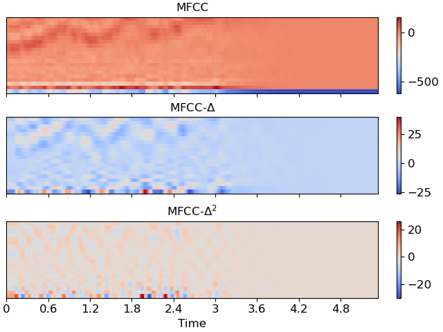
Compute MFCC deltas, delta-deltas

>>> y, sr = librosa.load(librosa.ex('trumpet'))
>>> mfcc = librosa.feature.mfcc(y=y, sr=sr)
>>> mfcc_delta = librosa.feature.delta(mfcc)
>>> mfcc_delta
array([[-1.610e+01, -1.610e+01, ...,  3.980e-14,  3.980e-14],
       [ 2.067e+00,  2.067e+00, ...,  0.000e+00,  0.000e+00],
       ...,
       [ 2.073e+00,  2.073e+00, ...,  0.000e+00,  0.000e+00],
       [-2.241e+00, -2.241e+00, ...,  0.000e+00,  0.000e+00]],
      dtype=float32)

>>> mfcc_delta2 = librosa.feature.delta(mfcc, order=2)
>>> mfcc_delta2
array([[1.088e+01, 1.088e+01, ..., 3.146e-14, 3.146e-14],
       [8.505e+00, 8.505e+00, ..., 0.000e+00, 0.000e+00],
       ...,
       [1.059e+00, 1.059e+00, ..., 0.000e+00, 0.000e+00],
       [3.197e+00, 3.197e+00, ..., 0.000e+00, 0.000e+00]],
      dtype=float32)

>>> import matplotlib.pyplot as plt
>>> fig, ax = plt.subplots(nrows=3, sharex=True, sharey=True)
>>> img1 = librosa.display.specshow(mfcc, ax=ax[0], x_axis='time')
>>> ax[0].set(title='MFCC')
>>> ax[0].label_outer()
>>> img2 = librosa.display.specshow(mfcc_delta, ax=ax[1], x_axis='time')
>>> ax[1].set(title=r'MFCC-$\Delta$')
>>> ax[1].label_outer()
>>> img3 = librosa.display.specshow(mfcc_delta2, ax=ax[2], x_axis='time')
>>> ax[2].set(title=r'MFCC-$\Delta^2$')
>>> fig.colorbar(img1, ax=[ax[0]])
>>> fig.colorbar(img2, ax=[ax[1]])
>>> fig.colorbar(img3, ax=[ax[2]])