Caution

You're reading an old version of this documentation. If you want up-to-date information, please have a look at 0.10.1.

librosa.perceptual_weighting

librosa.perceptual_weighting(S, frequencies, kind='A', **kwargs)

Perceptual weighting of a power spectrogram:

S_p[f] = frequency_weighting(f, 'A') + 10*log(S[f] / ref)

Parameters:

Snp.ndarray [shape=(d, t)]

Power spectrogram

frequenciesnp.ndarray [shape=(d,)]

Center frequency for each row of` S`

kindstr

The frequency weighting curve to use. e.g. ‘A’, ‘B’, ‘C’, ‘D’, None or ‘Z’

kwargsadditional keyword arguments

Additional keyword arguments to power_to_db.

Returns:

S_pnp.ndarray [shape=(d, t)]

perceptually weighted version of S

See also

power_to_db

Notes

This function caches at level 30.

Examples

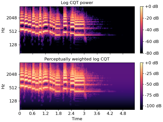
Re-weight a CQT power spectrum, using peak power as reference

>>> y, sr = librosa.load(librosa.ex('trumpet'))
>>> C = np.abs(librosa.cqt(y, sr=sr, fmin=librosa.note_to_hz('A1')))
>>> freqs = librosa.cqt_frequencies(C.shape[0],
...                                 fmin=librosa.note_to_hz('A1'))
>>> perceptual_CQT = librosa.perceptual_weighting(C**2,
...                                               freqs,
...                                               ref=np.max)
>>> perceptual_CQT
array([[ -96.528,  -97.101, ..., -108.561, -108.561],
       [ -95.88 ,  -96.479, ..., -107.551, -107.551],
       ...,
       [ -65.142,  -53.256, ...,  -80.098,  -80.098],
       [ -71.542,  -53.197, ...,  -80.311,  -80.311]])

>>> import matplotlib.pyplot as plt
>>> fig, ax = plt.subplots(nrows=2, sharex=True, sharey=True)
>>> img = librosa.display.specshow(librosa.amplitude_to_db(C,
...                                                        ref=np.max),
...                                fmin=librosa.note_to_hz('A1'),
...                                y_axis='cqt_hz', x_axis='time',
...                                ax=ax[0])
>>> ax[0].set(title='Log CQT power')
>>> ax[0].label_outer()
>>> imgp = librosa.display.specshow(perceptual_CQT, y_axis='cqt_hz',
...                                 fmin=librosa.note_to_hz('A1'),
...                                 x_axis='time', ax=ax[1])
>>> ax[1].set(title='Perceptually weighted log CQT')
>>> fig.colorbar(img, ax=ax[0], format="%+2.0f dB")
>>> fig.colorbar(imgp, ax=ax[1], format="%+2.0f dB")