librosa.feature.mfcc#

librosa.feature.mfcc(*, y=None, sr=22050, S=None, n_mfcc=20, dct_type=2, norm='ortho', lifter=0, mel_norm='slaney', ref=1.0, top_db=80.0, **kwargs)[source]#

Mel-frequency cepstral coefficients (MFCCs)

Parameters:

ynp.ndarray [shape=(…, n,)] or None

audio time series. Multi-channel is supported..

srnumber > 0 [scalar]

sampling rate of y

Snp.ndarray [shape=(…, d, t)] or None

log-power Mel spectrogram

n_mfccint > 0 [scalar]

number of MFCCs to return

dct_type{1, 2, 3}

Discrete cosine transform (DCT) type. By default, DCT type-2 is used.

normNone or ‘ortho’

If dct_type is 2 or 3, setting norm='ortho' uses an ortho-normal DCT basis. Normalization is not supported for dct_type=1.

lifternumber >= 0

If lifter>0, apply liftering (cepstral filtering) to the MFCCs::: M[n, :] <- M[n, :] * (1 + sin(pi * (n + 1) / lifter) * lifter / 2)

Setting lifter >= 2 * n_mfcc emphasizes the higher-order coefficients. As lifter increases, the coefficient weighting becomes approximately linear.

mel_normfloat, ‘slaney’, or None

norm argument to melspectrogram

reffloat or callable

Reference value for the log conversion, as in power_to_db. A scalar leaves each frame independent of the others. A callable such as np.max is evaluated over the frequency and time axes of each leading channel, which makes every frame’s output depend on every other frame in that channel.

This applies only when computing from y; if S is supplied it is assumed to already be in dB.

top_dbfloat or None

Threshold the mel spectrogram at top_db below its peak before the log conversion, as in power_to_db. The peak is computed over the frequency and time axes, independently for each leading channel, so a numeric value makes each frame’s output depend on every other frame in the same channel. Pass None to disable the threshold and make the result depend only on the frame itself.

**kwargs

additional keyword arguments to melspectrogram if operating on time series input

n_fftint > 0 [scalar]

length of the FFT frame

hop_lengthint > 0 [scalar]

number of samples between successive frames. See librosa.stft

win_lengthint <= n_fft [scalar]

Each frame of audio is windowed by window(). The window will be of length win_length and then padded with zeros to match n_fft. If unspecified, defaults to win_length = n_fft.

windowstr, tuple, number, function, or np.ndarray [shape=(n_fft,)]

a window specification (str, tuple, or number); see scipy.signal.get_window
a window function, such as scipy.signal.windows.hann
a vector or array of length n_fft

centerbool

If True, the signal y is padded so that frame t is centered at y[t * hop_length].
If False, then frame t begins at y[t * hop_length]

pad_modestr

If center=True, the padding mode to use at the edges of the signal. By default, STFT uses zero padding.

powerfloat > 0 [scalar]

Exponent applied to the spectrum before calculating the melspectrogram when the input is a time signal, e.g. 1 for magnitude, 2 for power (default), etc.

**kwargs

additional keyword arguments for Mel filter bank parameters

n_melsint > 0 [scalar]

number of Mel bands to generate

fminfloat >= 0 [scalar]

lowest frequency (in Hz)

fmaxfloat >= 0 [scalar]

highest frequency (in Hz). If None, use fmax = sr / 2.0

htkbool [scalar]

use HTK formula instead of Slaney

dtypenp.dtype

The data type of the output basis. By default, uses 32-bit (single-precision) floating point.

Returns:

Mnp.ndarray [shape=(…, n_mfcc, t)]: MFCC sequence

See also

melspectrogram
scipy.fft.dct

Examples

Generate mfccs from a time series

>>> y, sr = librosa.loadx('libri1')
>>> librosa.feature.mfcc(y=y, sr=sr)
array([[-565.919, -564.288, ..., -426.484, -434.668],
       [  10.305,   12.509, ...,   88.43 ,   90.12 ],
       ...,
       [   2.807,    2.068, ...,   -6.725,   -5.159],
       [   2.822,    2.244, ...,   -6.198,   -6.177]], dtype=float32)

Using a different hop length and HTK-style Mel frequencies

>>> librosa.feature.mfcc(y=y, sr=sr, hop_length=1024, htk=True)
array([[-5.471e+02, -5.464e+02, ..., -4.446e+02, -4.200e+02],
       [ 1.361e+01,  1.402e+01, ...,  9.764e+01,  9.869e+01],
       ...,
       [ 4.097e-01, -2.029e+00, ..., -1.051e+01, -1.130e+01],
       [-1.119e-01, -1.688e+00, ..., -3.442e+00, -4.687e+00]],
      dtype=float32)

Use a pre-computed log-power Mel spectrogram

>>> S = librosa.feature.melspectrogram(y=y, sr=sr, n_mels=128,
...                                    fmax=8000)
>>> librosa.feature.mfcc(S=librosa.power_to_db(S))
array([[-559.974, -558.449, ..., -411.96 , -420.458],
       [  11.018,   13.046, ...,   76.972,   80.888],
       ...,
       [   2.713,    2.379, ...,    1.464,   -2.835],
       [   2.712,    2.619, ...,    2.209,    0.648]], dtype=float32)

Get more components

>>> mfccs = librosa.feature.mfcc(y=y, sr=sr, n_mfcc=40)

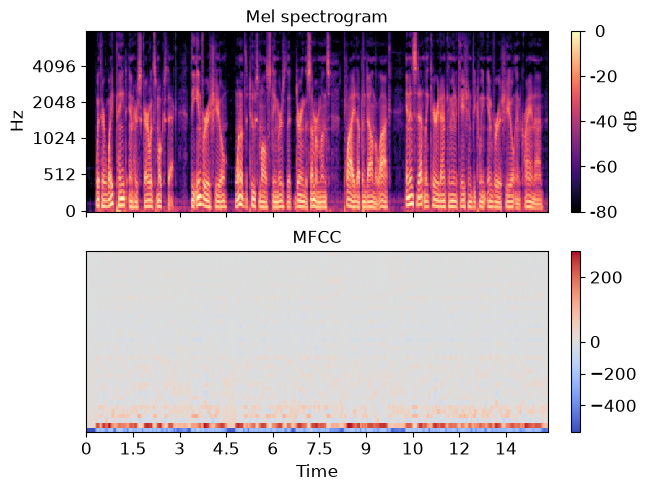
Visualize the MFCC series

>>> import matplotlib.pyplot as plt
>>> fig, ax = plt.subplots(nrows=2, sharex=True)
>>> img = librosa.display.specshow(S, vscale='dBFS[power]',
...                                x_axis='time', y_axis='mel', fmax=8000,
...                                ax=ax[0])
>>> librosa.display.colorbar_db(img)
>>> ax[0].set(title='Mel spectrogram')
>>> ax[0].label_outer()
>>> img = librosa.display.specshow(mfccs, x_axis='time', ax=ax[1])
>>> fig.colorbar(img, ax=[ax[1]])
>>> ax[1].set(title='MFCC')
>>> plt.show()

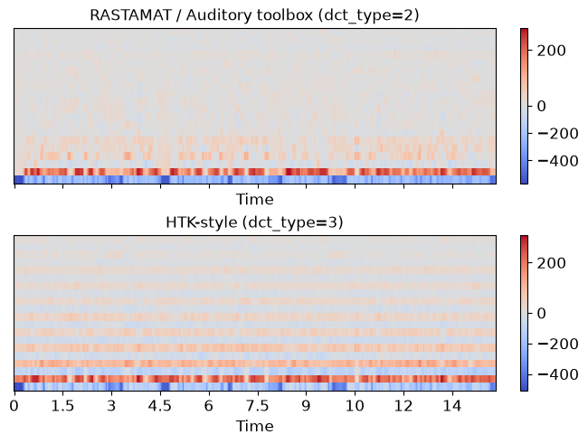
../../_images/librosa-feature-mfcc-1_00_00.png

Compare different DCT bases

>>> m_slaney = librosa.feature.mfcc(y=y, sr=sr, dct_type=2)
>>> m_htk = librosa.feature.mfcc(y=y, sr=sr, dct_type=3)
>>> fig, ax = plt.subplots(nrows=2, sharex=True, sharey=True, layout='compressed')
>>> img1 = librosa.display.specshow(m_slaney, x_axis='time', ax=ax[0])
>>> ax[0].set(title='RASTAMAT / Auditory toolbox (dct_type=2)')
>>> fig.colorbar(img, ax=[ax[0]])
>>> img2 = librosa.display.specshow(m_htk, x_axis='time', ax=ax[1])
>>> ax[1].set(title='HTK-style (dct_type=3)')
>>> fig.colorbar(img2, ax=[ax[1]])
>>> plt.show()

../../_images/librosa-feature-mfcc-1_01_00.png