Caution

You're reading an old version of this documentation. If you want up-to-date information, please have a look at 0.9.1.

Harmonic-percussive source separation

This notebook illustrates how to separate an audio signal into its harmonic and percussive components.

We’ll compare the original median-filtering based approach of Fitzgerald, 2010 and its margin-based extension due to Dreidger, Mueller and Disch, 2014.

from __future__ import print_function
import numpy as np
import matplotlib.pyplot as plt

import librosa
import librosa.display

Load the example clip.

y, sr = librosa.load('audio/Karissa_Hobbs_-_09_-_Lets_Go_Fishin.mp3', offset=40, duration=10)

Out:

/tmp/tmpfl4ra6qp/b0064fe7dbe8048b1d4148e61a568b6fe3fca91b/librosa/core/audio.py:161: UserWarning: PySoundFile failed. Trying audioread instead.
  warnings.warn('PySoundFile failed. Trying audioread instead.')

Compute the short-time Fourier transform of y

D = librosa.stft(y)

Decompose D into harmonic and percussive components

\(D = D_\text{harmonic} + D_\text{percussive}\)

D_harmonic, D_percussive = librosa.decompose.hpss(D)

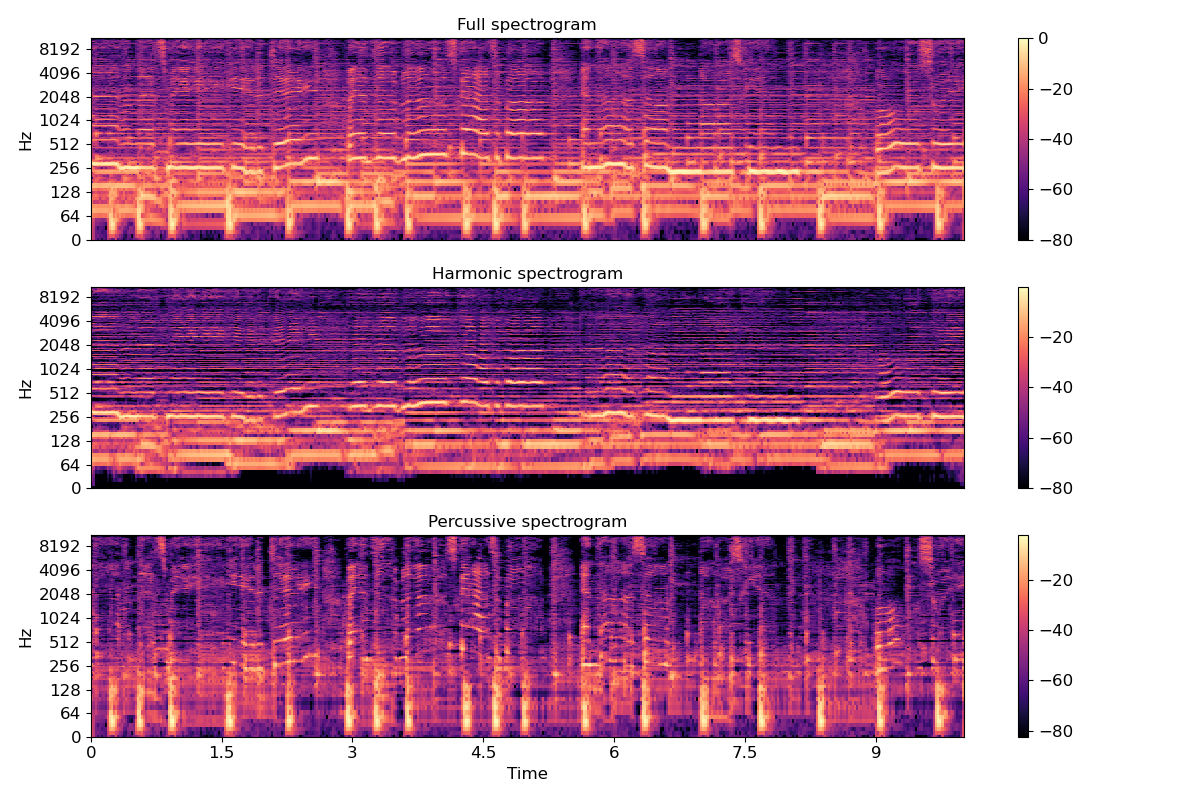
We can plot the two components along with the original spectrogram

# Pre-compute a global reference power from the input spectrum
rp = np.max(np.abs(D))

plt.figure(figsize=(12, 8))

plt.subplot(3, 1, 1)
librosa.display.specshow(librosa.amplitude_to_db(np.abs(D), ref=rp), y_axis='log')
plt.colorbar()
plt.title('Full spectrogram')

plt.subplot(3, 1, 2)
librosa.display.specshow(librosa.amplitude_to_db(np.abs(D_harmonic), ref=rp), y_axis='log')
plt.colorbar()
plt.title('Harmonic spectrogram')

plt.subplot(3, 1, 3)
librosa.display.specshow(librosa.amplitude_to_db(np.abs(D_percussive), ref=rp), y_axis='log', x_axis='time')
plt.colorbar()
plt.title('Percussive spectrogram')
plt.tight_layout()

Out:

/tmp/tmpfl4ra6qp/b0064fe7dbe8048b1d4148e61a568b6fe3fca91b/librosa/display.py:862: MatplotlibDeprecationWarning: The 'basey' parameter of __init__() has been renamed 'base' since Matplotlib 3.3; support for the old name will be dropped two minor releases later.
  scaler(mode, **kwargs)
/tmp/tmpfl4ra6qp/b0064fe7dbe8048b1d4148e61a568b6fe3fca91b/librosa/display.py:862: MatplotlibDeprecationWarning: The 'linthreshy' parameter of __init__() has been renamed 'linthresh' since Matplotlib 3.3; support for the old name will be dropped two minor releases later.
  scaler(mode, **kwargs)
/tmp/tmpfl4ra6qp/b0064fe7dbe8048b1d4148e61a568b6fe3fca91b/librosa/display.py:862: MatplotlibDeprecationWarning: The 'linscaley' parameter of __init__() has been renamed 'linscale' since Matplotlib 3.3; support for the old name will be dropped two minor releases later.
  scaler(mode, **kwargs)

The default HPSS above assigns energy to each time-frequency bin according to whether a horizontal (harmonic) or vertical (percussive) filter responds higher at that position.

This assumes that all energy belongs to either a harmonic or percussive source, but does not handle “noise” well. Noise energy ends up getting spread between D_harmonic and D_percussive.

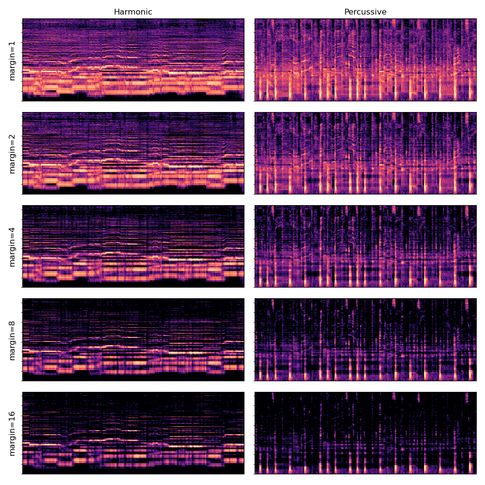
If we instead require that the horizontal filter responds more than the vertical filter by at least some margin, and vice versa, then noise can be removed from both components.

Note: the default (above) corresponds to margin=1

# Let's compute separations for a few different margins and compare the results below
D_harmonic2, D_percussive2 = librosa.decompose.hpss(D, margin=2)
D_harmonic4, D_percussive4 = librosa.decompose.hpss(D, margin=4)
D_harmonic8, D_percussive8 = librosa.decompose.hpss(D, margin=8)
D_harmonic16, D_percussive16 = librosa.decompose.hpss(D, margin=16)

In the plots below, note that vibrato has been suppressed from the harmonic components, and vocals have been suppressed in the percussive components.

plt.figure(figsize=(10, 10))

plt.subplot(5, 2, 1)
librosa.display.specshow(librosa.amplitude_to_db(np.abs(D_harmonic), ref=rp), y_axis='log')
plt.title('Harmonic')
plt.yticks([])
plt.ylabel('margin=1')

plt.subplot(5, 2, 2)
librosa.display.specshow(librosa.amplitude_to_db(np.abs(D_percussive), ref=rp), y_axis='log')
plt.title('Percussive')
plt.yticks([]), plt.ylabel('')

plt.subplot(5, 2, 3)
librosa.display.specshow(librosa.amplitude_to_db(np.abs(D_harmonic2), ref=rp), y_axis='log')
plt.yticks([])
plt.ylabel('margin=2')

plt.subplot(5, 2, 4)
librosa.display.specshow(librosa.amplitude_to_db(np.abs(D_percussive2), ref=rp), y_axis='log')
plt.yticks([]) ,plt.ylabel('')

plt.subplot(5, 2, 5)
librosa.display.specshow(librosa.amplitude_to_db(np.abs(D_harmonic4), ref=rp), y_axis='log')
plt.yticks([])
plt.ylabel('margin=4')

plt.subplot(5, 2, 6)
librosa.display.specshow(librosa.amplitude_to_db(np.abs(D_percussive4), ref=rp), y_axis='log')
plt.yticks([]), plt.ylabel('')

plt.subplot(5, 2, 7)
librosa.display.specshow(librosa.amplitude_to_db(np.abs(D_harmonic8), ref=rp), y_axis='log')
plt.yticks([])
plt.ylabel('margin=8')

plt.subplot(5, 2, 8)
librosa.display.specshow(librosa.amplitude_to_db(np.abs(D_percussive8), ref=rp), y_axis='log')
plt.yticks([]), plt.ylabel('')

plt.subplot(5, 2, 9)
librosa.display.specshow(librosa.amplitude_to_db(np.abs(D_harmonic16), ref=rp), y_axis='log')
plt.yticks([])
plt.ylabel('margin=16')

plt.subplot(5, 2, 10)
librosa.display.specshow(librosa.amplitude_to_db(np.abs(D_percussive16), ref=rp), y_axis='log')
plt.yticks([]), plt.ylabel('')

plt.tight_layout()
plt.show()

Out:

/tmp/tmpfl4ra6qp/b0064fe7dbe8048b1d4148e61a568b6fe3fca91b/librosa/display.py:862: MatplotlibDeprecationWarning: The 'basey' parameter of __init__() has been renamed 'base' since Matplotlib 3.3; support for the old name will be dropped two minor releases later.
  scaler(mode, **kwargs)
/tmp/tmpfl4ra6qp/b0064fe7dbe8048b1d4148e61a568b6fe3fca91b/librosa/display.py:862: MatplotlibDeprecationWarning: The 'linthreshy' parameter of __init__() has been renamed 'linthresh' since Matplotlib 3.3; support for the old name will be dropped two minor releases later.
  scaler(mode, **kwargs)
/tmp/tmpfl4ra6qp/b0064fe7dbe8048b1d4148e61a568b6fe3fca91b/librosa/display.py:862: MatplotlibDeprecationWarning: The 'linscaley' parameter of __init__() has been renamed 'linscale' since Matplotlib 3.3; support for the old name will be dropped two minor releases later.
  scaler(mode, **kwargs)