Caution

You're reading an old version of this documentation. If you want up-to-date information, please have a look at 0.9.1.

librosa.core.perceptual_weighting

librosa.core.perceptual_weighting(S, frequencies, **kwargs)

Perceptual weighting of a power spectrogram:

S_p[f] = A_weighting(f) + 10*log(S[f] / ref)

Parameters

Snp.ndarray [shape=(d, t)]

Power spectrogram

frequenciesnp.ndarray [shape=(d,)]

Center frequency for each row of S

kwargsadditional keyword arguments

Additional keyword arguments to power_to_db.

Returns

S_pnp.ndarray [shape=(d, t)]

perceptually weighted version of S

See also

power_to_db

Notes

This function caches at level 30.

Examples

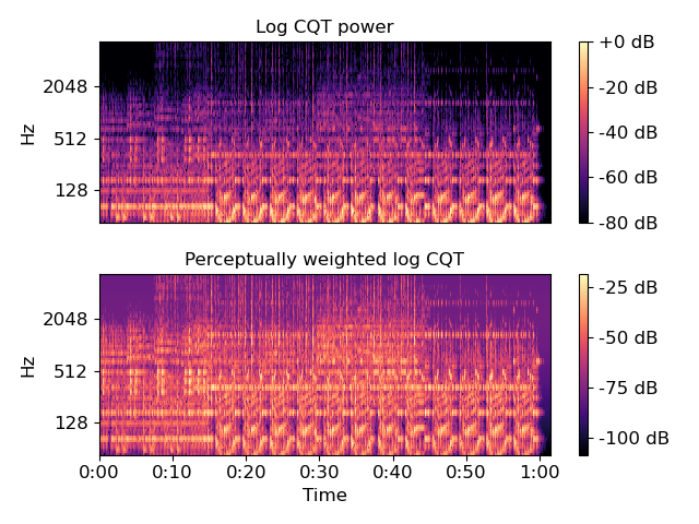
Re-weight a CQT power spectrum, using peak power as reference

>>> y, sr = librosa.load(librosa.util.example_audio_file())
>>> C = np.abs(librosa.cqt(y, sr=sr, fmin=librosa.note_to_hz('A1')))
>>> freqs = librosa.cqt_frequencies(C.shape[0],
...                                 fmin=librosa.note_to_hz('A1'))
>>> perceptual_CQT = librosa.perceptual_weighting(C**2,
...                                               freqs,
...                                               ref=np.max)
>>> perceptual_CQT
array([[ -80.076,  -80.049, ..., -104.735, -104.735],
       [ -78.344,  -78.555, ..., -103.725, -103.725],
       ...,
       [ -76.272,  -76.272, ...,  -76.272,  -76.272],
       [ -76.485,  -76.485, ...,  -76.485,  -76.485]])

>>> import matplotlib.pyplot as plt
>>> plt.figure()
>>> plt.subplot(2, 1, 1)
>>> librosa.display.specshow(librosa.amplitude_to_db(C,
...                                                  ref=np.max),
...                          fmin=librosa.note_to_hz('A1'),
...                          y_axis='cqt_hz')
>>> plt.title('Log CQT power')
>>> plt.colorbar(format='%+2.0f dB')
>>> plt.subplot(2, 1, 2)
>>> librosa.display.specshow(perceptual_CQT, y_axis='cqt_hz',
...                          fmin=librosa.note_to_hz('A1'),
...                          x_axis='time')
>>> plt.title('Perceptually weighted log CQT')
>>> plt.colorbar(format='%+2.0f dB')
>>> plt.tight_layout()
>>> plt.show()