Caution

You're reading an old version of this documentation. If you want up-to-date information, please have a look at 0.9.1.

librosa.display.waveplot

librosa.display.waveplot(y, sr=22050, max_points=50000.0, x_axis='time', offset=0.0, max_sr=1000, ax=None, **kwargs)

Plot the amplitude envelope of a waveform.

If y is monophonic, a filled curve is drawn between [-abs(y), abs(y)].

If y is stereo, the curve is drawn between [-abs(y[1]), abs(y[0])], so that the left and right channels are drawn above and below the axis, respectively.

Long signals (duration >= max_points) are down-sampled to at most max_sr before plotting.

Parameters

ynp.ndarray [shape=(n,) or (2,n)]

audio time series (mono or stereo)

srnumber > 0 [scalar]

sampling rate of y

max_pointspostive number or None

Maximum number of time-points to plot: if max_points exceeds the duration of y, then y is downsampled.

If None, no downsampling is performed.

x_axisstr or None

Display of the x-axis ticks and tick markers. Accepted values are:

• ‘time’markers are shown as milliseconds, seconds, minutes, or hours.

  Values are plotted in units of seconds.

• ‘s’ : markers are shown as seconds.

• ‘ms’ : markers are shown as milliseconds.

• ‘lag’ : like time, but past the halfway point counts as negative values.

• ‘lag_s’ : same as lag, but in seconds.

• ‘lag_ms’ : same as lag, but in milliseconds.

• None, ‘none’, or ‘off’: ticks and tick markers are hidden.

axmatplotlib.axes.Axes or None

Axes to plot on instead of the default plt.gca().

offsetfloat

Horizontal offset (in seconds) to start the waveform plot

max_srnumber > 0 [scalar]

Maximum sampling rate for the visualization

kwargs

Additional keyword arguments to matplotlib.pyplot.fill_between

Returns

pcmatplotlib.collections.PolyCollection

The PolyCollection created by fill_between.

See also

librosa.core.resample

matplotlib.pyplot.fill_between

Examples

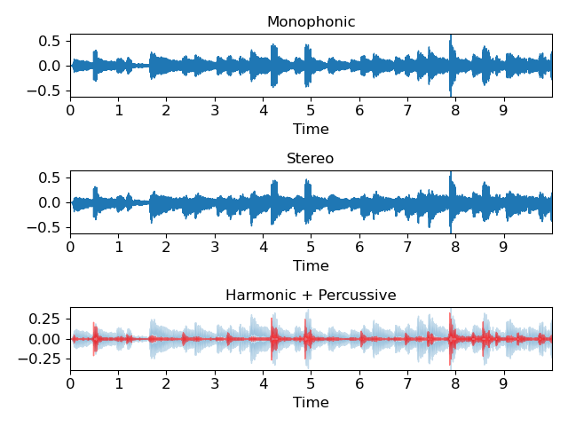
Plot a monophonic waveform

>>> import matplotlib.pyplot as plt
>>> y, sr = librosa.load(librosa.util.example_audio_file(), duration=10)
>>> plt.figure()
>>> plt.subplot(3, 1, 1)
>>> librosa.display.waveplot(y, sr=sr)
>>> plt.title('Monophonic')

Or a stereo waveform

>>> y, sr = librosa.load(librosa.util.example_audio_file(),
...                      mono=False, duration=10)
>>> plt.subplot(3, 1, 2)
>>> librosa.display.waveplot(y, sr=sr)
>>> plt.title('Stereo')

Or harmonic and percussive components with transparency

>>> y, sr = librosa.load(librosa.util.example_audio_file(), duration=10)
>>> y_harm, y_perc = librosa.effects.hpss(y)
>>> plt.subplot(3, 1, 3)
>>> librosa.display.waveplot(y_harm, sr=sr, alpha=0.25)
>>> librosa.display.waveplot(y_perc, sr=sr, color='r', alpha=0.5)
>>> plt.title('Harmonic + Percussive')
>>> plt.tight_layout()
>>> plt.show()