Caution

You're reading the documentation for a development version. For the latest released version, please have a look at 0.10.2.

librosa.feature.mfcc

librosa.feature.mfcc(*, y=None, sr=22050, S=None, n_mfcc=20, dct_type=2, norm='ortho', lifter=0, mel_norm='slaney', **kwargs)

Mel-frequency cepstral coefficients (MFCCs)

Warning

If multi-channel audio input y is provided, the MFCC calculation will depend on the peak loudness (in decibels) across all channels. The result may differ from independent MFCC calculation of each channel.

Parameters:

ynp.ndarray [shape=(…, n,)] or None

audio time series. Multi-channel is supported..

srnumber > 0 [scalar]

sampling rate of y

Snp.ndarray [shape=(…, d, t)] or None

log-power Mel spectrogram

n_mfccint > 0 [scalar]

number of MFCCs to return

dct_type{1, 2, 3}

Discrete cosine transform (DCT) type. By default, DCT type-2 is used.

normNone or ‘ortho’

If dct_type is 2 or 3, setting norm='ortho' uses an ortho-normal DCT basis. Normalization is not supported for dct_type=1.

lifternumber >= 0

If lifter>0, apply liftering (cepstral filtering) to the MFCCs::

M[n, :] <- M[n, :] * (1 + sin(pi * (n + 1) / lifter) * lifter / 2)

Setting lifter >= 2 * n_mfcc emphasizes the higher-order coefficients. As lifter increases, the coefficient weighting becomes approximately linear.

mel_normnorm argument to melspectrogram

**kwargsadditional keyword arguments to melspectrogram

if operating on time series input

n_fftint > 0 [scalar]

length of the FFT window

hop_lengthint > 0 [scalar]

number of samples between successive frames. See librosa.stft

win_lengthint <= n_fft [scalar]

Each frame of audio is windowed by window(). The window will be of length win_length and then padded with zeros to match n_fft. If unspecified, defaults to win_length = n_fft.

windowstring, tuple, number, function, or np.ndarray [shape=(n_fft,)]

• a window specification (string, tuple, or number);

see scipy.signal.get_window - a window function, such as scipy.signal.windows.hann - a vector or array of length n_fft .. see also:: librosa.filters.get_window

centerboolean

• If True, the signal y is padded so that frame

t is centered at y[t * hop_length]. - If False, then frame t begins at y[t * hop_length]

pad_modestring

If center=True, the padding mode to use at the edges of the signal. By default, STFT uses zero padding.

powerfloat > 0 [scalar]

Exponent applied to the spectrum before calculating the melspectrogram when the input is a time signal, e.g. 1 for magnitude, 2 for power (default), etc.

**kwargsadditional keyword arguments for Mel filter bank parameters

n_melsint > 0 [scalar]

number of Mel bands to generate

fminfloat >= 0 [scalar]

lowest frequency (in Hz)

fmaxfloat >= 0 [scalar]

highest frequency (in Hz). If None, use fmax = sr / 2.0

htkbool [scalar]

use HTK formula instead of Slaney

dtypenp.dtype

The data type of the output basis. By default, uses 32-bit (single-precision) floating point.

Returns:

Mnp.ndarray [shape=(…, n_mfcc, t)]

MFCC sequence

See also

melspectrogram

scipy.fftpack.dct

Examples

Generate mfccs from a time series

>>> y, sr = librosa.load(librosa.ex('libri1'))
>>> librosa.feature.mfcc(y=y, sr=sr)
array([[-565.919, -564.288, ..., -426.484, -434.668],
       [  10.305,   12.509, ...,   88.43 ,   90.12 ],
       ...,
       [   2.807,    2.068, ...,   -6.725,   -5.159],
       [   2.822,    2.244, ...,   -6.198,   -6.177]], dtype=float32)

Using a different hop length and HTK-style Mel frequencies

>>> librosa.feature.mfcc(y=y, sr=sr, hop_length=1024, htk=True)
array([[-5.471e+02, -5.464e+02, ..., -4.446e+02, -4.200e+02],
       [ 1.361e+01,  1.402e+01, ...,  9.764e+01,  9.869e+01],
       ...,
       [ 4.097e-01, -2.029e+00, ..., -1.051e+01, -1.130e+01],
       [-1.119e-01, -1.688e+00, ..., -3.442e+00, -4.687e+00]],
      dtype=float32)

Use a pre-computed log-power Mel spectrogram

>>> S = librosa.feature.melspectrogram(y=y, sr=sr, n_mels=128,
...                                    fmax=8000)
>>> librosa.feature.mfcc(S=librosa.power_to_db(S))
array([[-559.974, -558.449, ..., -411.96 , -420.458],
       [  11.018,   13.046, ...,   76.972,   80.888],
       ...,
       [   2.713,    2.379, ...,    1.464,   -2.835],
       [   2.712,    2.619, ...,    2.209,    0.648]], dtype=float32)

Get more components

>>> mfccs = librosa.feature.mfcc(y=y, sr=sr, n_mfcc=40)

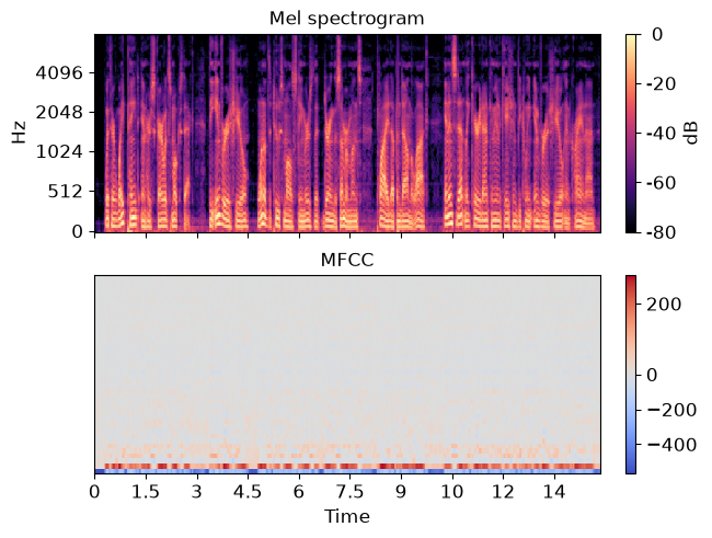
Visualize the MFCC series

>>> import matplotlib.pyplot as plt
>>> fig, ax = plt.subplots(nrows=2, sharex=True)
>>> img = librosa.display.specshow(librosa.power_to_db(S, ref=np.max),
...                                x_axis='time', y_axis='mel', fmax=8000,
...                                ax=ax[0])
>>> fig.colorbar(img, ax=[ax[0]])
>>> ax[0].set(title='Mel spectrogram')
>>> ax[0].label_outer()
>>> img = librosa.display.specshow(mfccs, x_axis='time', ax=ax[1])
>>> fig.colorbar(img, ax=[ax[1]])
>>> ax[1].set(title='MFCC')

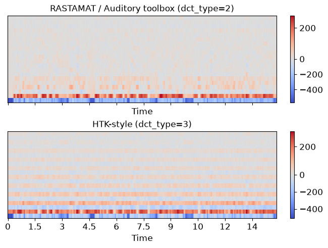
Compare different DCT bases

>>> m_slaney = librosa.feature.mfcc(y=y, sr=sr, dct_type=2)
>>> m_htk = librosa.feature.mfcc(y=y, sr=sr, dct_type=3)
>>> fig, ax = plt.subplots(nrows=2, sharex=True, sharey=True)
>>> img1 = librosa.display.specshow(m_slaney, x_axis='time', ax=ax[0])
>>> ax[0].set(title='RASTAMAT / Auditory toolbox (dct_type=2)')
>>> fig.colorbar(img, ax=[ax[0]])
>>> img2 = librosa.display.specshow(m_htk, x_axis='time', ax=ax[1])
>>> ax[1].set(title='HTK-style (dct_type=3)')
>>> fig.colorbar(img2, ax=[ax[1]])