Caution

You're reading an old version of this documentation. If you want up-to-date information, please have a look at 0.10.2.

Harmonic-percussive source separation

This notebook illustrates how to separate an audio signal into its harmonic and percussive components.

We’ll compare the original median-filtering based approach of Fitzgerald, 2010 and its margin-based extension due to Dreidger, Mueller and Disch, 2014.

import numpy as np
import matplotlib.pyplot as plt

from IPython.display import Audio

import librosa

Load an example clip with harmonics and percussives

y, sr = librosa.load(librosa.ex('fishin'), duration=5, offset=10)

Audio(data=y, rate=sr)

Compute the short-time Fourier transform of y

D = librosa.stft(y)

Decompose D into harmonic and percussive components

\(D = D_\text{harmonic} + D_\text{percussive}\)

D_harmonic, D_percussive = librosa.decompose.hpss(D)

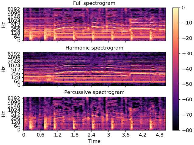
We can plot the two components along with the original spectrogram

# Pre-compute a global reference power from the input spectrum
rp = np.max(np.abs(D))

fig, ax = plt.subplots(nrows=3, sharex=True, sharey=True)

img = librosa.display.specshow(librosa.amplitude_to_db(np.abs(D), ref=rp),
                         y_axis='log', x_axis='time', ax=ax[0])
ax[0].set(title='Full spectrogram')
ax[0].label_outer()

librosa.display.specshow(librosa.amplitude_to_db(np.abs(D_harmonic), ref=rp),
                         y_axis='log', x_axis='time', ax=ax[1])
ax[1].set(title='Harmonic spectrogram')
ax[1].label_outer()

librosa.display.specshow(librosa.amplitude_to_db(np.abs(D_percussive), ref=rp),
                         y_axis='log', x_axis='time', ax=ax[2])
ax[2].set(title='Percussive spectrogram')
fig.colorbar(img, ax=ax)

We can also invert the separated spectrograms to play back the audio. First the harmonic signal:

y_harmonic = librosa.istft(D_harmonic, length=len(y))
Audio(data=y_harmonic, rate=sr)

And next the percussive signal:

y_percussive = librosa.istft(D_percussive, length=len(y))
Audio(data=y_percussive, rate=sr)

The default HPSS above assigns energy to each time-frequency bin according to whether a horizontal (harmonic) or vertical (percussive) filter responds higher at that position.

This assumes that all energy belongs to either a harmonic or percussive source, but does not handle “noise” well. Noise energy ends up getting spread between D_harmonic and D_percussive. Unfortunately, this often also includes vocals and other sounds that are not purely harmonic or percussive.

If we instead require that the horizontal filter responds more than the vertical filter by at least some margin, and vice versa, then noise can be removed from both components.

Note: the default (above) corresponds to margin=1

# Let's compute separations for a few different margins and compare the results below
D_harmonic2, D_percussive2 = librosa.decompose.hpss(D, margin=2)
D_harmonic4, D_percussive4 = librosa.decompose.hpss(D, margin=4)
D_harmonic8, D_percussive8 = librosa.decompose.hpss(D, margin=8)
D_harmonic16, D_percussive16 = librosa.decompose.hpss(D, margin=16)

In the plots below, note that vibrato has been suppressed from the harmonic components, and vocals have been suppressed in the percussive components.

fig, ax = plt.subplots(nrows=5, ncols=2, sharex=True, sharey=True, figsize=(10, 10))
librosa.display.specshow(librosa.amplitude_to_db(np.abs(D_harmonic), ref=rp),
                         y_axis='log', x_axis='time', ax=ax[0, 0])
ax[0, 0].set(title='Harmonic')

librosa.display.specshow(librosa.amplitude_to_db(np.abs(D_percussive), ref=rp),
                         y_axis='log', x_axis='time', ax=ax[0, 1])
ax[0, 1].set(title='Percussive')

librosa.display.specshow(librosa.amplitude_to_db(np.abs(D_harmonic2), ref=rp),
                         y_axis='log', x_axis='time', ax=ax[1, 0])

librosa.display.specshow(librosa.amplitude_to_db(np.abs(D_percussive2), ref=rp),
                         y_axis='log', x_axis='time', ax=ax[1, 1])

librosa.display.specshow(librosa.amplitude_to_db(np.abs(D_harmonic4), ref=rp),
                         y_axis='log', x_axis='time', ax=ax[2, 0])

librosa.display.specshow(librosa.amplitude_to_db(np.abs(D_percussive4), ref=rp),
                         y_axis='log', x_axis='time', ax=ax[2, 1])

librosa.display.specshow(librosa.amplitude_to_db(np.abs(D_harmonic8), ref=rp),
                         y_axis='log', x_axis='time', ax=ax[3, 0])

librosa.display.specshow(librosa.amplitude_to_db(np.abs(D_percussive8), ref=rp),
                         y_axis='log', x_axis='time', ax=ax[3, 1])

librosa.display.specshow(librosa.amplitude_to_db(np.abs(D_harmonic16), ref=rp),
                         y_axis='log', x_axis='time', ax=ax[4, 0])

librosa.display.specshow(librosa.amplitude_to_db(np.abs(D_percussive16), ref=rp),
                         y_axis='log', x_axis='time', ax=ax[4, 1])

for i in range(5):
    ax[i, 0].set(ylabel='margin={:d}'.format(2**i))
    ax[i, 0].label_outer()
    ax[i, 1].label_outer()

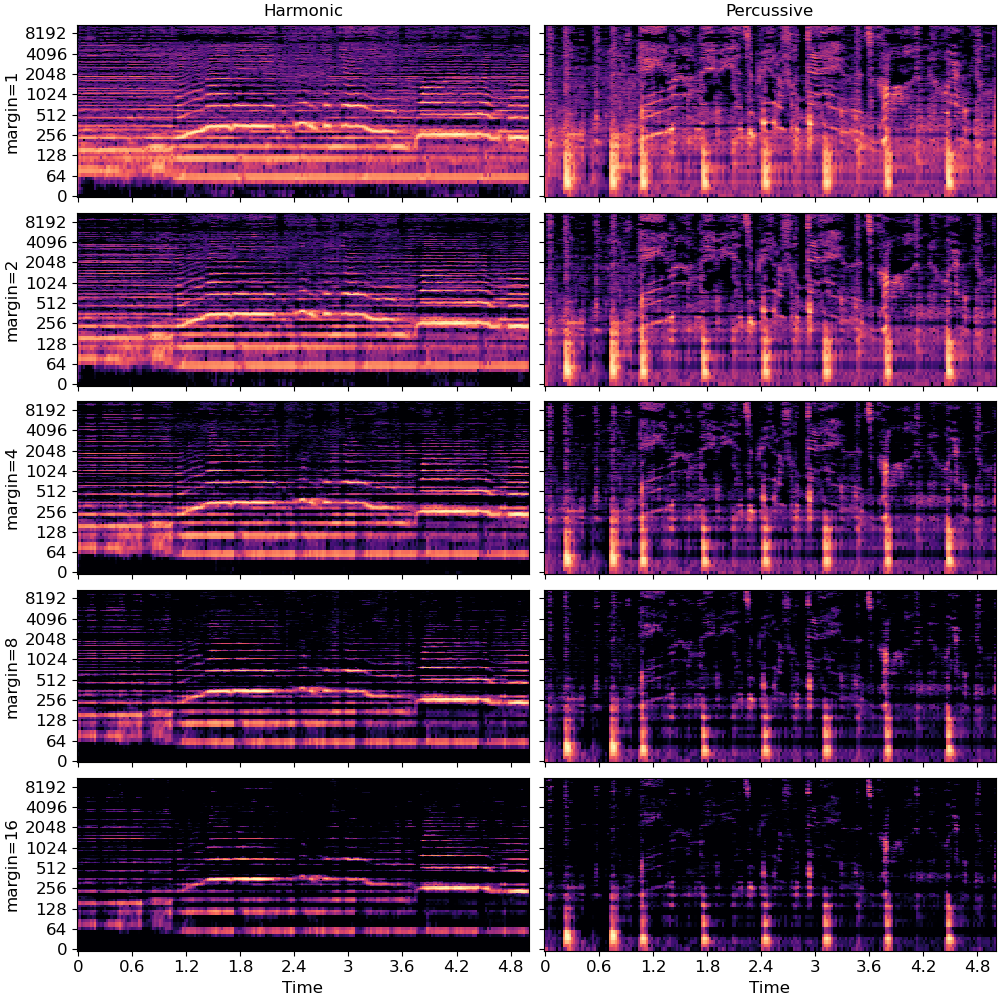
In the plots above, it looks like margins of 4 or greater are sufficient to produce strictly harmonic and percussive components.

We can invert and play those components back just as before. Again, starting with the harmonic component:

y_harmonic4 = librosa.istft(D_harmonic4, length=len(y))
Audio(data=y_harmonic4, rate=sr)

And the percussive component:

y_percussive4 = librosa.istft(D_percussive4, length=len(y))
Audio(data=y_percussive4, rate=sr)