Caution
You're reading an old version of this documentation. If you want up-to-date information, please have a look at 0.10.2.
librosa.display.specshow
- librosa.display.specshow(data, *, x_coords=None, y_coords=None, x_axis=None, y_axis=None, sr=22050, hop_length=512, n_fft=None, win_length=None, fmin=None, fmax=None, tuning=0.0, bins_per_octave=12, key='C:maj', Sa=None, mela=None, thaat=None, auto_aspect=True, htk=False, unicode=True, intervals=None, unison=None, ax=None, **kwargs)[source]
Display a spectrogram/chromagram/cqt/etc.
For a detailed overview of this function, see Using display.specshow
- Parameters:
- datanp.ndarray [shape=(d, n)]
Matrix to display (e.g., spectrogram)
- srnumber > 0 [scalar]
Sample rate used to determine time scale in x-axis.
- hop_lengthint > 0 [scalar]
Hop length, also used to determine time scale in x-axis
- n_fftint > 0 or None
Number of samples per frame in STFT/spectrogram displays. By default, this will be inferred from the shape of
dataas2 * (d - 1). Ifdatawas generated using an odd frame length, the correct value can be specified here.- win_lengthint > 0 or None
The number of samples per window. By default, this will be inferred to match
n_fft. This is primarily useful for specifying odd window lengths in Fourier tempogram displays.- x_axis, y_axisNone or str
Range for the x- and y-axes.
Valid types are:
None, ‘none’, or ‘off’ : no axis decoration is displayed.
Frequency types:
‘linear’, ‘fft’, ‘hz’ : frequency range is determined by the FFT window and sampling rate.
‘log’ : the spectrum is displayed on a log scale.
‘fft_note’: the spectrum is displayed on a log scale with pitches marked.
‘fft_svara’: the spectrum is displayed on a log scale with svara marked.
‘mel’ : frequencies are determined by the mel scale.
‘cqt_hz’ : frequencies are determined by the CQT scale.
‘cqt_note’ : pitches are determined by the CQT scale.
‘cqt_svara’ : like cqt_note but using Hindustani or Carnatic svara
‘vqt_fjs’ : like cqt_note but using Functional Just System (FJS) notation. This requires a just intonation-based variable-Q transform representation.
All frequency types are plotted in units of Hz.
Any spectrogram parameters (hop_length, sr, bins_per_octave, etc.) used to generate the input data should also be provided when calling
specshow.Categorical types:
‘chroma’ : pitches are determined by the chroma filters. Pitch classes are arranged at integer locations (0-11) according to a given key.
chroma_h, chroma_c: pitches are determined by chroma filters, and labeled as svara in the Hindustani (chroma_h) or Carnatic (chroma_c) according to a given thaat (Hindustani) or melakarta raga (Carnatic).
‘chroma_fjs’: pitches are determined by chroma filters using just intonation. All pitch classes are annotated.
‘tonnetz’ : axes are labeled by Tonnetz dimensions (0-5)
‘frames’ : markers are shown as frame counts.
Time types:
- ‘time’markers are shown as milliseconds, seconds, minutes, or hours.
Values are plotted in units of seconds.
‘h’ : markers are shown as hours, minutes, and seconds.
‘m’ : markers are shown as minutes and seconds.
‘s’ : markers are shown as seconds.
‘ms’ : markers are shown as milliseconds.
‘lag’ : like time, but past the halfway point counts as negative values.
‘lag_h’ : same as lag, but in hours, minutes and seconds.
‘lag_m’ : same as lag, but in minutes and seconds.
‘lag_s’ : same as lag, but in seconds.
‘lag_ms’ : same as lag, but in milliseconds.
Rhythm:
- ‘tempo’markers are shown as beats-per-minute (BPM)
using a logarithmic scale. This is useful for visualizing the outputs of feature.tempogram.
- ‘fourier_tempo’same as ‘tempo’, but used when
tempograms are calculated in the Frequency domain using feature.fourier_tempogram.
- x_coords, y_coordsnp.ndarray [shape=data.shape[0 or 1]]
Optional positioning coordinates of the input data. These can be use to explicitly set the location of each element
data[i, j], e.g., for displaying beat-synchronous features in natural time coordinates.If not provided, they are inferred from
x_axisandy_axis.- fminfloat > 0 [scalar] or None
Frequency of the lowest spectrogram bin. Used for Mel, CQT, and VQT scales.
If
y_axisis cqt_hz or cqt_note andfminis not given, it is set by default tonote_to_hz('C1').- fmaxfloat > 0 [scalar] or None
Used for setting the Mel frequency scales
- tuningfloat
Tuning deviation from A440, in fractions of a bin.
This is used for CQT frequency scales, so that
fminis adjusted tofmin * 2**(tuning / bins_per_octave).- bins_per_octaveint > 0 [scalar]
Number of bins per octave. Used for CQT frequency scale.
- keystr
The reference key to use when using note axes (cqt_note, chroma).
- Safloat or int
If using Hindustani or Carnatic svara axis decorations, specify Sa.
For cqt_svara,
Sashould be specified as a frequency in Hz.For chroma_c or chroma_h,
Sashould correspond to the position of Sa within the chromagram. If not provided, Sa will default to 0 (equivalent to C)- melastr or int, optional
If using chroma_c or cqt_svara display mode, specify the melakarta raga.
- thaatstr, optional
If using chroma_h display mode, specify the parent thaat.
- intervalsstr or array of floats in [1, 2), optional
If using an FJS notation (chroma_fjs, vqt_fjs), the interval specification.
See
core.interval_frequenciesfor a description of supported values.- unisonstr, optional
If using an FJS notation (chroma_fjs, vqt_fjs), the pitch name of the unison interval. If not provided, it will be inferred from fmin (for VQT display) or assumed as ‘C’ (for chroma display).
- auto_aspectbool
Axes will have ‘equal’ aspect if the horizontal and vertical dimensions cover the same extent and their types match.
To override, set to False.
- htkbool
If plotting on a mel frequency axis, specify which version of the mel scale to use.
False: use Slaney formula (default)
True: use HTK formula
See
core.mel_frequenciesfor more information.- unicodebool
If using note or svara decorations, setting unicode=True will use unicode glyphs for accidentals and octave encoding.
Setting unicode=False will use ASCII glyphs. This can be helpful if your font does not support musical notation symbols.
- axmatplotlib.axes.Axes or None
Axes to plot on instead of the default plt.gca().
- **kwargsadditional keyword arguments
Arguments passed through to
matplotlib.pyplot.pcolormesh.By default, the following options are set:
rasterized=Trueshading='auto'edgecolors='None'
The
cmapoption if not provided, is inferred from data automatically. Setcmap=Noneto use matplotlib’s default colormap.
- Returns:
- colormesh
matplotlib.collections.QuadMesh The color mesh object produced by
matplotlib.pyplot.pcolormesh
- colormesh
See also
cmapAutomatic colormap detection
matplotlib.pyplot.pcolormesh
Examples
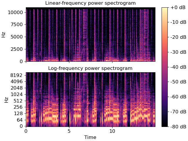
Visualize an STFT power spectrum using default parameters
>>> import matplotlib.pyplot as plt
>>> y, sr = librosa.load(librosa.ex('choice'), duration=15)
>>> fig, ax = plt.subplots(nrows=2, ncols=1, sharex=True)
>>> D = librosa.amplitude_to_db(np.abs(librosa.stft(y)), ref=np.max)
>>> img = librosa.display.specshow(D, y_axis='linear', x_axis='time',
...                                sr=sr, ax=ax[0])
>>> ax[0].set(title='Linear-frequency power spectrogram')
>>> ax[0].label_outer()
Or on a logarithmic scale, and using a larger hop
>>> hop_length = 1024
>>> D = librosa.amplitude_to_db(np.abs(librosa.stft(y, hop_length=hop_length)),
...                             ref=np.max)
>>> librosa.display.specshow(D, y_axis='log', sr=sr, hop_length=hop_length,
...                          x_axis='time', ax=ax[1])
>>> ax[1].set(title='Log-frequency power spectrogram')
>>> ax[1].label_outer()
>>> fig.colorbar(img, ax=ax, format="%+2.f dB")