Caution

You're reading an old version of this documentation. If you want up-to-date information, please have a look at 0.10.2.

librosa.segment.agglomerative

librosa.segment.agglomerative(data, k, clusterer=None, axis=-1)

Bottom-up temporal segmentation.

Use a temporally-constrained agglomerative clustering routine to partition data into k contiguous segments.

Parameters:

datanp.ndarray

data to cluster

kint > 0 [scalar]

number of segments to produce

clusterersklearn.cluster.AgglomerativeClustering, optional

An optional AgglomerativeClustering object. If None, a constrained Ward object is instantiated.

axisint

axis along which to cluster. By default, the last axis (-1) is chosen.

Returns:

boundariesnp.ndarray [shape=(k,)]

left-boundaries (frame numbers) of detected segments. This will always include 0 as the first left-boundary.

See also

sklearn.cluster.AgglomerativeClustering

Examples

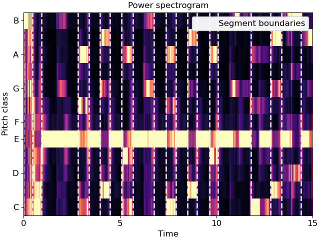
Cluster by chroma similarity, break into 20 segments

>>> y, sr = librosa.load(librosa.ex('nutcracker'), duration=15)
>>> chroma = librosa.feature.chroma_cqt(y=y, sr=sr)
>>> bounds = librosa.segment.agglomerative(chroma, 20)
>>> bound_times = librosa.frames_to_time(bounds, sr=sr)
>>> bound_times
array([ 0.   ,  0.65 ,  1.091,  1.927,  2.438,  2.902,  3.924,
        4.783,  5.294,  5.712,  6.13 ,  7.314,  8.522,  8.916,
        9.66 , 10.844, 11.238, 12.028, 12.492, 14.095])

Plot the segmentation over the chromagram

>>> import matplotlib.pyplot as plt
>>> fig, ax = plt.subplots()
>>> librosa.display.specshow(chroma, y_axis='chroma', x_axis='time', ax=ax)
>>> ax.vlines(bound_times, 0, chroma.shape[0], color='linen', linestyle='--',
...           linewidth=2, alpha=0.9, label='Segment boundaries')
>>> ax.legend()
>>> ax.set(title='Power spectrogram')