Caution

You're reading an old version of this documentation. If you want up-to-date information, please have a look at 0.10.2.

librosa.beat.plp

librosa.beat.plp(*, y=None, sr=22050, onset_envelope=None, hop_length=512, win_length=384, tempo_min=30, tempo_max=300, prior=None)

Predominant local pulse (PLP) estimation. [1]

The PLP method analyzes the onset strength envelope in the frequency domain to find a locally stable tempo for each frame. These local periodicities are used to synthesize local half-waves, which are combined such that peaks coincide with rhythmically salient frames (e.g. onset events on a musical time grid). The local maxima of the pulse curve can be taken as estimated beat positions.

This method may be preferred over the dynamic programming method of beat_track when either the tempo is expected to vary significantly over time. Additionally, since plp does not require the entire signal to make predictions, it may be preferable when beat-tracking long recordings in a streaming setting.

[1]

Grosche, P., & Muller, M. (2011). “Extracting predominant local pulse information from music recordings.” IEEE Transactions on Audio, Speech, and Language Processing, 19(6), 1688-1701.

Parameters:

ynp.ndarray [shape=(…, n)] or None

audio time series. Multi-channel is supported.

srnumber > 0 [scalar]

sampling rate of y

onset_envelopenp.ndarray [shape=(…, n)] or None

(optional) pre-computed onset strength envelope

hop_lengthint > 0 [scalar]

number of audio samples between successive onset_envelope values

win_lengthint > 0 [scalar]

number of frames to use for tempogram analysis. By default, 384 frames (at sr=22050 and hop_length=512) corresponds to about 8.9 seconds.

tempo_min, tempo_maxnumbers > 0 [scalar], optional

Minimum and maximum permissible tempo values. tempo_max must be at least tempo_min.

Set either (or both) to None to disable this constraint.

priorscipy.stats.rv_continuous [optional]

A prior distribution over tempo (in beats per minute). By default, a uniform prior over [tempo_min, tempo_max] is used.

Returns:

pulsenp.ndarray, shape=[(…, n)]

The estimated pulse curve. Maxima correspond to rhythmically salient points of time.

If input is multi-channel, one pulse curve per channel is computed.

See also

beat_track

librosa.onset.onset_strength

librosa.feature.fourier_tempogram

Examples

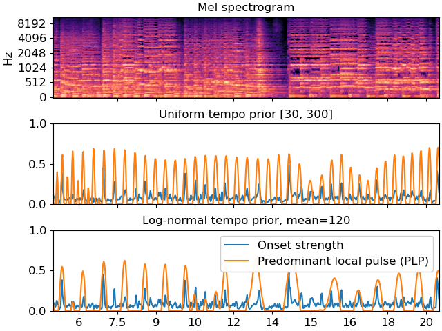
Visualize the PLP compared to an onset strength envelope. Both are normalized here to make comparison easier.

>>> y, sr = librosa.load(librosa.ex('brahms'))
>>> onset_env = librosa.onset.onset_strength(y=y, sr=sr)
>>> pulse = librosa.beat.plp(onset_envelope=onset_env, sr=sr)
>>> # Or compute pulse with an alternate prior, like log-normal
>>> import scipy.stats
>>> prior = scipy.stats.lognorm(loc=np.log(120), scale=120, s=1)
>>> pulse_lognorm = librosa.beat.plp(onset_envelope=onset_env, sr=sr,
...                                  prior=prior)
>>> melspec = librosa.feature.melspectrogram(y=y, sr=sr)

>>> import matplotlib.pyplot as plt
>>> fig, ax = plt.subplots(nrows=3, sharex=True)
>>> librosa.display.specshow(librosa.power_to_db(melspec,
...                                              ref=np.max),
...                          x_axis='time', y_axis='mel', ax=ax[0])
>>> ax[0].set(title='Mel spectrogram')
>>> ax[0].label_outer()
>>> ax[1].plot(librosa.times_like(onset_env),
...          librosa.util.normalize(onset_env),
...          label='Onset strength')
>>> ax[1].plot(librosa.times_like(pulse),
...          librosa.util.normalize(pulse),
...          label='Predominant local pulse (PLP)')
>>> ax[1].set(title='Uniform tempo prior [30, 300]')
>>> ax[1].label_outer()
>>> ax[2].plot(librosa.times_like(onset_env),
...          librosa.util.normalize(onset_env),
...          label='Onset strength')
>>> ax[2].plot(librosa.times_like(pulse_lognorm),
...          librosa.util.normalize(pulse_lognorm),
...          label='Predominant local pulse (PLP)')
>>> ax[2].set(title='Log-normal tempo prior, mean=120', xlim=[5, 20])
>>> ax[2].legend()

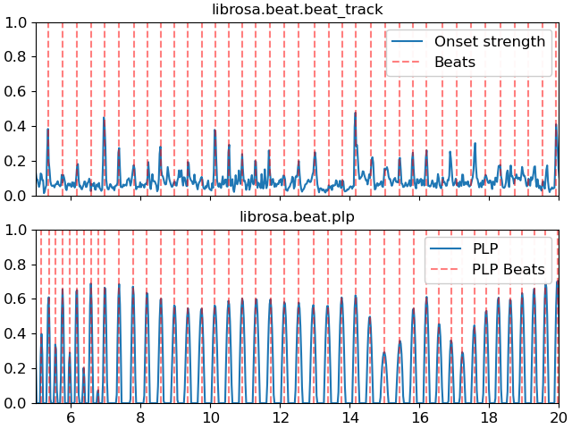
PLP local maxima can be used as estimates of beat positions.

>>> tempo, beats = librosa.beat.beat_track(onset_envelope=onset_env)
>>> beats_plp = np.flatnonzero(librosa.util.localmax(pulse))
>>> import matplotlib.pyplot as plt
>>> fig, ax = plt.subplots(nrows=2, sharex=True, sharey=True)
>>> times = librosa.times_like(onset_env, sr=sr)
>>> ax[0].plot(times, librosa.util.normalize(onset_env),
...          label='Onset strength')
>>> ax[0].vlines(times[beats], 0, 1, alpha=0.5, color='r',
...            linestyle='--', label='Beats')
>>> ax[0].legend()
>>> ax[0].set(title='librosa.beat.beat_track')
>>> ax[0].label_outer()
>>> # Limit the plot to a 15-second window
>>> times = librosa.times_like(pulse, sr=sr)
>>> ax[1].plot(times, librosa.util.normalize(pulse),
...          label='PLP')
>>> ax[1].vlines(times[beats_plp], 0, 1, alpha=0.5, color='r',
...            linestyle='--', label='PLP Beats')
>>> ax[1].legend()
>>> ax[1].set(title='librosa.beat.plp', xlim=[5, 20])
>>> ax[1].xaxis.set_major_formatter(librosa.display.TimeFormatter())