Caution

You're reading an old version of this documentation. If you want up-to-date information, please have a look at 0.10.2.

librosa.feature.inverse.mel_to_stft

librosa.feature.inverse.mel_to_stft(M, *, sr=22050, n_fft=2048, power=2.0, **kwargs)

Approximate STFT magnitude from a Mel power spectrogram.

Parameters:

Mnp.ndarray [shape=(…, n_mels, n), non-negative]

The spectrogram as produced by feature.melspectrogram

srnumber > 0 [scalar]

sampling rate of the underlying signal

n_fftint > 0 [scalar]

number of FFT components in the resulting STFT

powerfloat > 0 [scalar]

Exponent for the magnitude melspectrogram

**kwargsadditional keyword arguments

Mel filter bank parameters. See librosa.filters.mel for details

Returns:

Snp.ndarray [shape=(…, n_fft, t), non-negative]

An approximate linear magnitude spectrogram

See also

librosa.feature.melspectrogram

librosa.stft

librosa.filters.mel

librosa.util.nnls

Examples

>>> y, sr = librosa.load(librosa.ex('trumpet'))
>>> S = np.abs(librosa.stft(y))
>>> mel_spec = librosa.feature.melspectrogram(S=S, sr=sr)
>>> S_inv = librosa.feature.inverse.mel_to_stft(mel_spec, sr=sr)

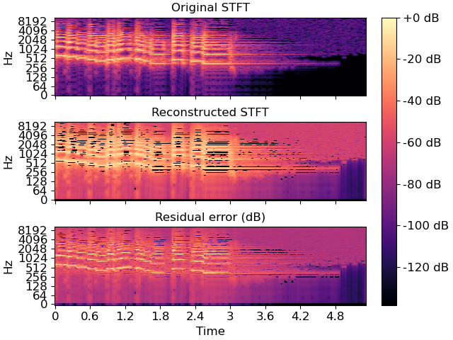
Compare the results visually

>>> import matplotlib.pyplot as plt
>>> fig, ax = plt.subplots(nrows=3, sharex=True, sharey=True)
>>> img = librosa.display.specshow(librosa.amplitude_to_db(S, ref=np.max, top_db=None),
...                          y_axis='log', x_axis='time', ax=ax[0])
>>> ax[0].set(title='Original STFT')
>>> ax[0].label_outer()
>>> librosa.display.specshow(librosa.amplitude_to_db(S_inv, ref=np.max, top_db=None),
...                          y_axis='log', x_axis='time', ax=ax[1])
>>> ax[1].set(title='Reconstructed STFT')
>>> ax[1].label_outer()
>>> librosa.display.specshow(librosa.amplitude_to_db(np.abs(S_inv - S),
...                                                  ref=S.max(), top_db=None),
...                          vmax=0, y_axis='log', x_axis='time', cmap='magma', ax=ax[2])
>>> ax[2].set(title='Residual error (dB)')
>>> fig.colorbar(img, ax=ax, format="%+2.f dB")