Caution

You're reading the documentation for a development version. For the latest released version, please have a look at 0.11.0.

librosa.display.waveshow

librosa.display.waveshow(y, *, sr=22050, max_points=11025, axis='time', offset=0.0, marker='', where='post', label=None, transpose=False, mask=None, ax=None, invert=False, invert_color=None, **kwargs)

Visualize a waveform in the time domain.

This function constructs a plot which adaptively switches between a raw samples-based view of the signal (matplotlib.pyplot.step) and an amplitude-envelope view of the signal (matplotlib.pyplot.fill_between) depending on the time extent of the plot’s viewport.

More specifically, when the plot spans a time interval of less than max_points / sr (by default, 1/2 second), the samples-based view is used, and otherwise a downsampled amplitude envelope is used. This is done to limit the complexity of the visual elements to guarantee an efficient, visually interpretable plot.

When using interactive rendering (e.g., in a Jupyter notebook or IPython console), the plot will automatically update as the view-port is changed, either through widget controls or programmatic updates.

Note

When visualizing stereo waveforms, the amplitude envelope will be generated so that the upper limits derive from the left channel, and the lower limits derive from the right channel, which can produce a vertically asymmetric plot.

When zoomed in to the sample view, only the first channel will be shown. If you want to visualize both channels at the sample level, it is recommended to plot each signal independently.

To visualize stereo waveforms as two separate signal displays, see multiplot.

Parameters:

ynp.ndarray [shape=(n,) or (2,n)]

audio time series (mono or stereo) If stereo, the left channel’s amplitude envelope will be used for the top of the plot,, and the right channel’s amplitude envelope (negated) will be used for the bottom of the plot. If mono, the signal’s envelope is mirrored across the axis.

srnumber > 0 [scalar]

sampling rate of y (samples per second)

max_pointsint > 0

Maximum number of samples to draw. When the plot covers a time extent smaller than max_points / sr (default: 1/2 second), samples are drawn.

If drawing raw samples would exceed max_points, then a downsampled amplitude envelope extracted from non-overlapping windows of y is visualized instead. The parameters of the amplitude envelope are defined so that the resulting plot cannot produce more than max_points frames.

axisstr or None

Display style of the axis ticks and tick markers. Accepted values are:

• ‘time’markers are shown as milliseconds, seconds, minutes, or hours.

  Values are plotted in units of seconds.

• ‘h’ : markers are shown as hours, minutes, and seconds.

• ‘m’ : markers are shown as minutes and seconds.

• ‘s’ : markers are shown as seconds.

• ‘ms’ : markers are shown as milliseconds.

• ‘lag’ : like time, but past the halfway point counts as negative values.

• ‘lag_h’ : same as lag, but in hours.

• ‘lag_m’ : same as lag, but in minutes.

• ‘lag_s’ : same as lag, but in seconds.

• ‘lag_ms’ : same as lag, but in milliseconds.

• None, ‘none’, or ‘off’: ticks and tick markers are hidden.

offsetfloat

Offset (in seconds) to start the waveform plot

markerstr

Marker symbol to use for sample values. (default: no markers)

See Also: matplotlib.markers.

where{‘pre’, ‘mid’, ‘post’}

This setting determines how both waveform and envelope plots interpolate between observations.

See matplotlib.pyplot.step for details.

Default: ‘post’

labelstr or None

The label string applied to this plot. Note that the label

transposebool

If True, display the wave vertically instead of horizontally.

masknp.ndarray [shape=(n,)] or None

If provided, this mask will be used to determine which samples to display. The mask should be a 1D boolean array of the same length as y (y.shape[-1]), where True indicates that the sample should be displayed, and False indicates that it should be ignored.

Note

This mask is only used directly by the envelope display, and a raw sample display will not be masked. The mask parameter is intended to be used by the wavef0 function, and it is not recommended to be used directly by the user.

axmatplotlib.axes.Axes or None

Axes to plot on instead of the default plt.gca().

invertbool

If True, invert the foreground and background of the display, so that the axes background is colored. If False (default), the waveform display is colored and the background is unchanged.

Note

This option should only be used if the wave display is the only element in the axes.

invert_colorstr, tuple, None

If invert is True, this parameter specifies the color to use for the inverted waveform display. If None (default), the color is set to the current axes background color.

**kwargs

Additional keyword arguments to matplotlib.pyplot.fill_between and matplotlib.pyplot.step.

Note that only those arguments which are common to both functions will be supported.

Returns:

librosa.display.AdaptiveWaveplot

An object of type librosa.display.AdaptiveWaveplot

See also

wavebars

AdaptiveWaveplot

multiplot

matplotlib.pyplot.step

matplotlib.pyplot.fill_between

matplotlib.pyplot.fill_betweenx

matplotlib.markers

Examples

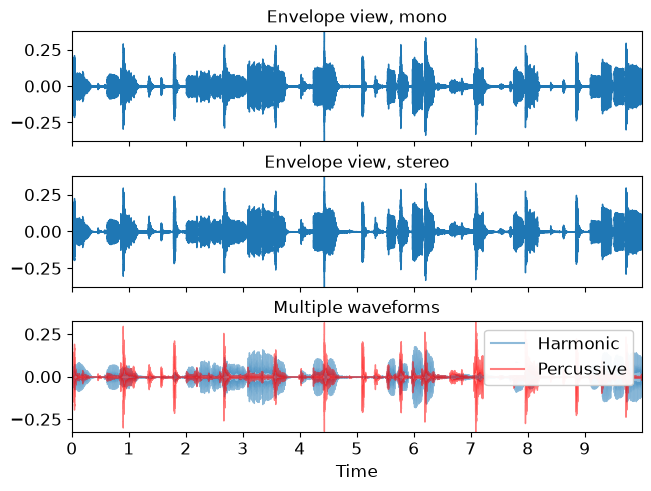
Plot a monophonic waveform with an envelope view

>>> import matplotlib.pyplot as plt
>>> y, sr = librosa.loadx('choice', duration=10)
>>> fig, ax = plt.subplots(nrows=3, sharex=True)
>>> librosa.display.waveshow(y, sr=sr, ax=ax[0])
>>> ax[0].set(title='Envelope view, mono')
>>> ax[0].label_outer()

Or a stereo waveform

>>> y, sr = librosa.loadx('choice', mono=False, duration=10)
>>> librosa.display.waveshow(y, sr=sr, ax=ax[1])
>>> ax[1].set(title='Envelope view, stereo')
>>> ax[1].label_outer()

Or harmonic and percussive components with transparency

>>> y, sr = librosa.loadx('choice', duration=10)
>>> y_harm, y_perc = librosa.effects.hpss(y)
>>> librosa.display.waveshow(y_harm, sr=sr, alpha=0.5, ax=ax[2], label='Harmonic')
>>> librosa.display.waveshow(y_perc, sr=sr, color='r', alpha=0.5, ax=ax[2], label='Percussive')
>>> ax[2].set(title='Multiple waveforms')
>>> ax[2].legend()
>>> plt.show()

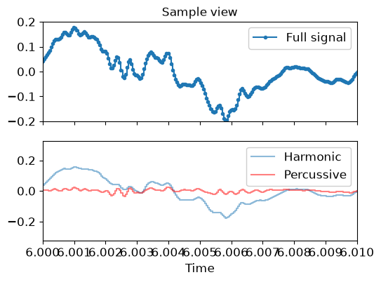
Zooming in on a plot to show raw sample values

>>> fig, (ax, ax2) = plt.subplots(nrows=2, sharex=True)
>>> ax.set(xlim=[6.0, 6.01], title='Sample view', ylim=[-0.2, 0.2])
>>> librosa.display.waveshow(y, sr=sr, ax=ax, marker='.', label='Full signal')
>>> librosa.display.waveshow(y_harm, sr=sr, alpha=0.5, ax=ax2, label='Harmonic')
>>> librosa.display.waveshow(y_perc, sr=sr, color='r', alpha=0.5, ax=ax2, label='Percussive')
>>> ax.label_outer()
>>> ax.legend()
>>> ax2.legend()
>>> plt.show()

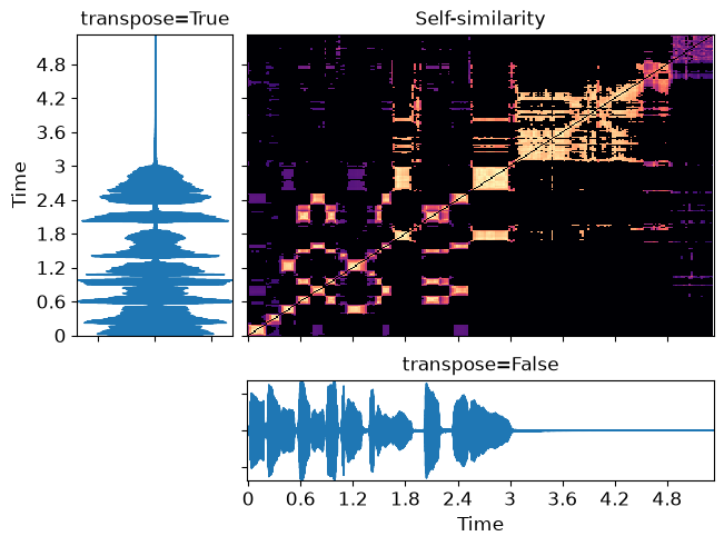
Plotting a transposed wave along with a self-similarity matrix

>>> fig, ax = plt.subplot_mosaic("hSSS;hSSS;hSSS;.vvv", layout='compressed')
>>> y, sr = librosa.loadx('trumpet')
>>> chroma = librosa.feature.chroma_cqt(y=y, sr=sr)
>>> sim = librosa.segment.recurrence_matrix(chroma, mode='affinity')
>>> librosa.display.specshow(sim, ax=ax['S'], sr=sr,
...                          x_axis='time', y_axis='time',
...                          auto_aspect=False)
>>> ax['S'].label_outer()
>>> ax['S'].sharex(ax['v'])
>>> ax['S'].sharey(ax['h'])
>>> ax['S'].set(title='Self-similarity')
>>> librosa.display.waveshow(y, ax=ax['v'])
>>> ax['v'].label_outer()
>>> ax['v'].set(title='transpose=False')
>>> librosa.display.waveshow(y, ax=ax['h'], transpose=True)
>>> ax['h'].label_outer()
>>> ax['h'].set(title='transpose=True')
>>> plt.show()