Caution

You're reading the documentation for a development version. For the latest released version, please have a look at 0.10.1.

librosa.feature.tempo

librosa.feature.tempo(*, y=None, sr=22050, onset_envelope=None, tg=None, hop_length=512, start_bpm=120, std_bpm=1.0, ac_size=8.0, max_tempo=320.0, aggregate=<function mean>, prior=None)

Estimate the tempo (beats per minute)

Parameters:

ynp.ndarray [shape=(…, n)] or None

audio time series. Multi-channel is supported.

srnumber > 0 [scalar]

sampling rate of the time series

onset_envelopenp.ndarray [shape=(…, n)]

pre-computed onset strength envelope

tgnp.ndarray

pre-computed tempogram. If provided, then y and onset_envelope are ignored, and win_length is inferred from the shape of the tempogram.

hop_lengthint > 0 [scalar]

hop length of the time series

start_bpmfloat [scalar]

initial guess of the BPM

std_bpmfloat > 0 [scalar]

standard deviation of tempo distribution

ac_sizefloat > 0 [scalar]

length (in seconds) of the auto-correlation window

max_tempofloat > 0 [scalar, optional]

If provided, only estimate tempo below this threshold

aggregatecallable [optional]

Aggregation function for estimating global tempo. If None, then tempo is estimated independently for each frame.

priorscipy.stats.rv_continuous [optional]

A prior distribution over tempo (in beats per minute). By default, a pseudo-log-normal prior is used. If given, start_bpm and std_bpm will be ignored.

Returns:

temponp.ndarray

estimated tempo (beats per minute). If input is multi-channel, one tempo estimate per channel is provided.

See also

librosa.onset.onset_strength

librosa.feature.tempogram

Notes

This function caches at level 30.

Examples

>>> # Estimate a static tempo
>>> y, sr = librosa.load(librosa.ex('nutcracker'), duration=30)
>>> onset_env = librosa.onset.onset_strength(y=y, sr=sr)
>>> tempo = librosa.feature.tempo(onset_envelope=onset_env, sr=sr)
>>> tempo
array([143.555])

>>> # Or a static tempo with a uniform prior instead
>>> import scipy.stats
>>> prior = scipy.stats.uniform(30, 300)  # uniform over 30-300 BPM
>>> utempo = librosa.feature.tempo(onset_envelope=onset_env, sr=sr, prior=prior)
>>> utempo
array([161.499])

>>> # Or a dynamic tempo
>>> dtempo = librosa.feature.tempo(onset_envelope=onset_env, sr=sr,
...                                aggregate=None)
>>> dtempo
array([ 89.103,  89.103,  89.103, ..., 123.047, 123.047, 123.047])

>>> # Dynamic tempo with a proper log-normal prior
>>> prior_lognorm = scipy.stats.lognorm(loc=np.log(120), scale=120, s=1)
>>> dtempo_lognorm = librosa.feature.tempo(onset_envelope=onset_env, sr=sr,
...                                        aggregate=None,
...                                        prior=prior_lognorm)
>>> dtempo_lognorm
array([ 89.103,  89.103,  89.103, ..., 123.047, 123.047, 123.047])

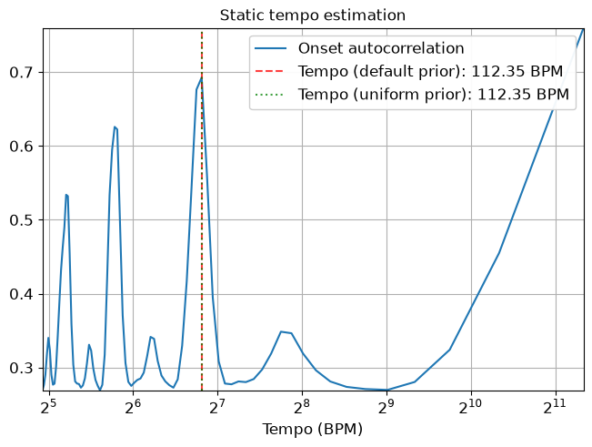
Plot the estimated tempo against the onset autocorrelation

>>> import matplotlib.pyplot as plt
>>> # Convert to scalar
>>> tempo = tempo.item()
>>> utempo = utempo.item()
>>> # Compute 2-second windowed autocorrelation
>>> hop_length = 512
>>> ac = librosa.autocorrelate(onset_env, max_size=2 * sr // hop_length)
>>> freqs = librosa.tempo_frequencies(len(ac), sr=sr,
...                                   hop_length=hop_length)
>>> # Plot on a BPM axis.  We skip the first (0-lag) bin.
>>> fig, ax = plt.subplots()
>>> ax.semilogx(freqs[1:], librosa.util.normalize(ac)[1:],
...              label='Onset autocorrelation', base=2)
>>> ax.axvline(tempo, 0, 1, alpha=0.75, linestyle='--', color='r',
...             label='Tempo (default prior): {:.2f} BPM'.format(tempo))
>>> ax.axvline(utempo, 0, 1, alpha=0.75, linestyle=':', color='g',
...             label='Tempo (uniform prior): {:.2f} BPM'.format(utempo))
>>> ax.set(xlabel='Tempo (BPM)', title='Static tempo estimation')
>>> ax.grid(True)
>>> ax.legend()

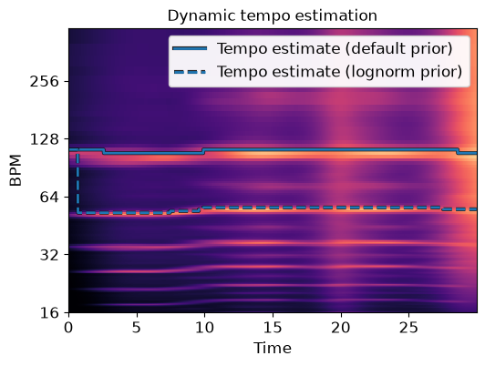
Plot dynamic tempo estimates over a tempogram

>>> fig, ax = plt.subplots()
>>> tg = librosa.feature.tempogram(onset_envelope=onset_env, sr=sr,
...                                hop_length=hop_length)
>>> librosa.display.specshow(tg, x_axis='time', y_axis='tempo', cmap='magma', ax=ax)
>>> ax.plot(librosa.times_like(dtempo), dtempo,
...          color='c', linewidth=1.5, label='Tempo estimate (default prior)')
>>> ax.plot(librosa.times_like(dtempo_lognorm), dtempo_lognorm,
...          color='c', linewidth=1.5, linestyle='--',
...          label='Tempo estimate (lognorm prior)')
>>> ax.set(title='Dynamic tempo estimation')
>>> ax.legend()