Caution

You're reading an old version of this documentation. If you want up-to-date information, please have a look at 0.9.1.

librosa.core.chirp

librosa.core.chirp(fmin, fmax, sr=22050, length=None, duration=None, linear=False, phi=None)

Returns a chirp signal that goes from frequency fmin to frequency fmax

Parameters

fminfloat > 0

initial frequency

fmaxfloat > 0

final frequency

srnumber > 0

desired sampling rate of the output signal

lengthint > 0

desired number of samples in the output signal. When both duration and length are defined, length would take priority.

durationfloat > 0

desired duration in seconds. When both duration and length are defined, length would take priority.

linearboolean

• If True, use a linear sweep, i.e., frequency changes linearly with time

• If False, use a exponential sweep.

Default is False.

phifloat or None

phase offset, in radians. If unspecified, defaults to -np.pi * 0.5.

Returns

chirp_signalnp.ndarray [shape=(length,), dtype=float64]

Synthesized chirp signal

Raises

ParameterError

• If either fmin or fmax are not provided.

• If neither length nor duration are provided.

See also

scipy.signal.chirp

Examples

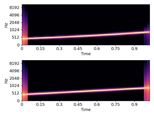
>>> # Generate a exponential chirp from A4 to A5
>>> exponential_chirp = librosa.chirp(440, 880, duration=1)

>>> # Or generate the same signal using `length`
>>> exponential_chirp = librosa.chirp(440, 880, sr=22050, length=22050)

>>> # Or generate a linear chirp instead
>>> linear_chirp = librosa.chirp(440, 880, duration=1, linear=True)

Display spectrogram for both exponential and linear chirps

>>> import matplotlib.pyplot as plt
>>> plt.figure()
>>> S_exponential = librosa.feature.melspectrogram(y=exponential_chirp)
>>> ax = plt.subplot(2,1,1)
>>> librosa.display.specshow(librosa.power_to_db(S_exponential, ref=np.max),
...                          x_axis='time', y_axis='mel')
>>> plt.subplot(2,1,2, sharex=ax)
>>> S_linear = librosa.feature.melspectrogram(y=linear_chirp)
>>> librosa.display.specshow(librosa.power_to_db(S_linear, ref=np.max),
...                          x_axis='time', y_axis='mel')
>>> plt.tight_layout()
>>> plt.show()