Caution

You're reading an old version of this documentation. If you want up-to-date information, please have a look at 0.9.1.

librosa.filters.constant_q

librosa.filters.constant_q(sr, fmin=None, n_bins=84, bins_per_octave=12, tuning=<DEPRECATED parameter>, window='hann', filter_scale=1, pad_fft=True, norm=1, dtype=<class 'numpy.complex64'>, **kwargs)

Construct a constant-Q basis.

This uses the filter bank described by [1].

1

McVicar, Matthew. “A machine learning approach to automatic chord extraction.” Dissertation, University of Bristol. 2013.

Parameters

srnumber > 0 [scalar]

Audio sampling rate

fminfloat > 0 [scalar]

Minimum frequency bin. Defaults to C1 ~= 32.70

n_binsint > 0 [scalar]

Number of frequencies. Defaults to 7 octaves (84 bins).

bins_per_octaveint > 0 [scalar]

Number of bins per octave

tuningfloat [scalar] <DEPRECATED>

Tuning deviation from A440 in fractions of a bin

Note

This parameter is deprecated in 0.7.1. It will be removed in version 0.8.

windowstring, tuple, number, or function

Windowing function to apply to filters.

filter_scalefloat > 0 [scalar]

Scale of filter windows. Small values (<1) use shorter windows for higher temporal resolution.

pad_fftboolean

Center-pad all filters up to the nearest integral power of 2.

By default, padding is done with zeros, but this can be overridden by setting the mode= field in kwargs.

norm{inf, -inf, 0, float > 0}

Type of norm to use for basis function normalization. See librosa.util.normalize

dtypenp.dtype

The data type of the output basis. By default, uses 64-bit (single precision) complex floating point.

kwargsadditional keyword arguments

Arguments to np.pad() when pad==True.

Returns

filtersnp.ndarray, len(filters) == n_bins

filters[i] is ith time-domain CQT basis filter

lengthsnp.ndarray, len(lengths) == n_bins

The (fractional) length of each filter

See also

constant_q_lengths

librosa.core.cqt

librosa.util.normalize

Notes

This function caches at level 10.

Examples

Use a shorter window for each filter

>>> basis, lengths = librosa.filters.constant_q(22050, filter_scale=0.5)

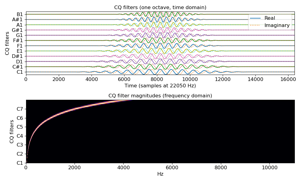
Plot one octave of filters in time and frequency

>>> import matplotlib.pyplot as plt
>>> basis, lengths = librosa.filters.constant_q(22050)
>>> plt.figure(figsize=(10, 6))
>>> plt.subplot(2, 1, 1)
>>> notes = librosa.midi_to_note(np.arange(24, 24 + len(basis)))
>>> for i, (f, n) in enumerate(zip(basis, notes[:12])):
...     f_scale = librosa.util.normalize(f) / 2
...     plt.plot(i + f_scale.real)
...     plt.plot(i + f_scale.imag, linestyle=':')
>>> plt.axis('tight')
>>> plt.yticks(np.arange(len(notes[:12])), notes[:12])
>>> plt.ylabel('CQ filters')
>>> plt.title('CQ filters (one octave, time domain)')
>>> plt.xlabel('Time (samples at 22050 Hz)')
>>> plt.legend(['Real', 'Imaginary'], frameon=True, framealpha=0.8)
>>> plt.subplot(2, 1, 2)
>>> F = np.abs(np.fft.fftn(basis, axes=[-1]))
>>> # Keep only the positive frequencies
>>> F = F[:, :(1 + F.shape[1] // 2)]
>>> librosa.display.specshow(F, x_axis='linear')
>>> plt.yticks(np.arange(len(notes))[::12], notes[::12])
>>> plt.ylabel('CQ filters')
>>> plt.title('CQ filter magnitudes (frequency domain)')
>>> plt.tight_layout()
>>> plt.show()