Caution

You're reading an old version of this documentation. If you want up-to-date information, please have a look at 0.10.1.

librosa.feature.mfcc

librosa.feature.mfcc(y=None, sr=22050, S=None, n_mfcc=20, dct_type=2, norm='ortho', lifter=0, **kwargs)

Mel-frequency cepstral coefficients (MFCCs)

Parameters:

ynp.ndarray [shape=(n,)] or None

audio time series

srnumber > 0 [scalar]

sampling rate of y

Snp.ndarray [shape=(d, t)] or None

log-power Mel spectrogram

n_mfcc: int > 0 [scalar]

number of MFCCs to return

dct_type{1, 2, 3}

Discrete cosine transform (DCT) type. By default, DCT type-2 is used.

normNone or ‘ortho’

If dct_type is 2 or 3, setting norm='ortho' uses an ortho-normal DCT basis.

Normalization is not supported for dct_type=1.

lifternumber >= 0

If lifter>0, apply liftering (cepstral filtering) to the MFCCs:

M[n, :] <- M[n, :] * (1 + sin(pi * (n + 1) / lifter) * lifter / 2)

Setting lifter >= 2 * n_mfcc emphasizes the higher-order coefficients. As lifter increases, the coefficient weighting becomes approximately linear.

kwargsadditional keyword arguments

Arguments to melspectrogram, if operating on time series input

Returns:

Mnp.ndarray [shape=(n_mfcc, t)]

MFCC sequence

See also

melspectrogram

scipy.fftpack.dct

Examples

Generate mfccs from a time series

>>> y, sr = librosa.load(librosa.ex('trumpet'))
>>> librosa.feature.mfcc(y=y, sr=sr)
array([[-249.124, -236.652, ..., -619.714, -619.714],
       [  73.787,   51.215, ...,    0.   ,    0.   ],
       ...,
       [ -10.144,   -9.091, ...,    0.   ,    0.   ],
       [ -13.994,  -21.184, ...,    0.   ,    0.   ]],
      dtype=float32)

Using a different hop length and HTK-style Mel frequencies

>>> librosa.feature.mfcc(y=y, sr=sr, hop_length=1024, htk=True)
array([[-274.064, -296.403, ..., -643.958, -643.958],
       [  63.888,    0.907, ...,    0.   ,    0.   ],
       ...,
       [  13.069,   36.896, ...,    0.   ,    0.   ],
       [  -2.986,  -13.714, ...,    0.   ,    0.   ]],
      dtype=float32)

Use a pre-computed log-power Mel spectrogram

>>> S = librosa.feature.melspectrogram(y=y, sr=sr, n_mels=128,
...                                    fmax=8000)
>>> librosa.feature.mfcc(S=librosa.power_to_db(S))
array([[-222.66 , -209.08 , ..., -627.181, -627.181],
       [  32.214,    2.315, ...,    0.   ,    0.   ],
       ...,
       [   0.872,   -4.195, ...,    0.   ,    0.   ],
       [  29.123,   33.193, ...,    0.   ,    0.   ]],
      dtype=float32)

Get more components

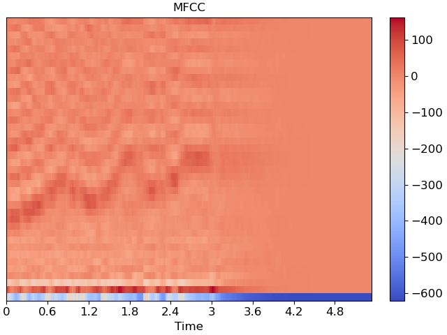
>>> mfccs = librosa.feature.mfcc(y=y, sr=sr, n_mfcc=40)

Visualize the MFCC series

>>> import matplotlib.pyplot as plt
>>> fig, ax = plt.subplots()
>>> img = librosa.display.specshow(mfccs, x_axis='time', ax=ax)
>>> fig.colorbar(img, ax=ax)
>>> ax.set(title='MFCC')

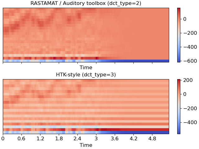
Compare different DCT bases

>>> m_slaney = librosa.feature.mfcc(y=y, sr=sr, dct_type=2)
>>> m_htk = librosa.feature.mfcc(y=y, sr=sr, dct_type=3)
>>> fig, ax = plt.subplots(nrows=2, sharex=True, sharey=True)
>>> img1 = librosa.display.specshow(m_slaney, x_axis='time', ax=ax[0])
>>> ax[0].set(title='RASTAMAT / Auditory toolbox (dct_type=2)')
>>> fig.colorbar(img, ax=[ax[0]])
>>> img2 = librosa.display.specshow(m_htk, x_axis='time', ax=ax[1])
>>> ax[1].set(title='HTK-style (dct_type=3)')
>>> fig.colorbar(img2, ax=[ax[1]])