Caution
You're reading an old version of this documentation. If you want up-to-date information, please have a look at 0.10.2.
librosa.feature.spectral_bandwidth
- librosa.feature.spectral_bandwidth(y=None, sr=22050, S=None, n_fft=2048, hop_length=512, win_length=None, window='hann', center=True, pad_mode='reflect', freq=None, centroid=None, norm=True, p=2)[source]
Compute p’th-order spectral bandwidth.
The spectral bandwidth [1] at frame
tis computed by:(sum_k S[k, t] * (freq[k, t] - centroid[t])**p)**(1/p)
- Parameters:
- ynp.ndarray [shape=(n,)] or None
audio time series
- srnumber > 0 [scalar]
audio sampling rate of
y- Snp.ndarray [shape=(d, t)] or None
(optional) spectrogram magnitude
- n_fftint > 0 [scalar]
FFT window size
- hop_lengthint > 0 [scalar]
hop length for STFT. See
librosa.stftfor details.- win_lengthint <= n_fft [scalar]
Each frame of audio is windowed by window(). The window will be of length
win_lengthand then padded with zeros to matchn_fft.If unspecified, defaults to
win_length = n_fft.- windowstring, tuple, number, function, or np.ndarray [shape=(n_fft,)]
a window specification (string, tuple, or number); see
scipy.signal.get_windowa window function, such as
scipy.signal.windows.hanna vector or array of length
n_fft
- centerboolean
If True, the signal
yis padded so that frametis centered aty[t * hop_length].If
False, then frametbegins aty[t * hop_length]
- pad_modestring
If
center=True, the padding mode to use at the edges of the signal. By default, STFT uses reflection padding.- freqNone or np.ndarray [shape=(d,) or shape=(d, t)]
Center frequencies for spectrogram bins.
If None, then FFT bin center frequencies are used. Otherwise, it can be a single array of
dcenter frequencies, or a matrix of center frequencies as constructed bylibrosa.reassigned_spectrogram- centroidNone or np.ndarray [shape=(1, t)]
pre-computed centroid frequencies
- normbool
Normalize per-frame spectral energy (sum to one)
- pfloat > 0
Power to raise deviation from spectral centroid.
- Returns:
- bandwidthnp.ndarray [shape=(1, t)]
frequency bandwidth for each frame
Examples
From time-series input
>>> y, sr = librosa.load(librosa.ex('trumpet'))
>>> spec_bw = librosa.feature.spectral_bandwidth(y=y, sr=sr)
>>> spec_bw
array([[1273.836, 1228.873, ..., 2952.357, 3013.68 ]])
From spectrogram input
>>> S, phase = librosa.magphase(librosa.stft(y=y))
>>> librosa.feature.spectral_bandwidth(S=S)
array([[1273.836, 1228.873, ..., 2952.357, 3013.68 ]])
Using variable bin center frequencies
>>> freqs, times, D = librosa.reassigned_spectrogram(y, fill_nan=True)
>>> librosa.feature.spectral_bandwidth(S=np.abs(D), freq=freqs)
array([[1274.637, 1228.786, ..., 2952.4  , 3013.735]])
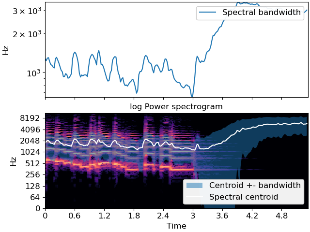
Plot the result
>>> import matplotlib.pyplot as plt
>>> fig, ax = plt.subplots(nrows=2, sharex=True)
>>> times = librosa.times_like(spec_bw)
>>> centroid = librosa.feature.spectral_centroid(S=S)
>>> ax[0].semilogy(times, spec_bw[0], label='Spectral bandwidth')
>>> ax[0].set(ylabel='Hz', xticks=[], xlim=[times.min(), times.max()])
>>> ax[0].legend()
>>> ax[0].label_outer()
>>> librosa.display.specshow(librosa.amplitude_to_db(S, ref=np.max),
...                          y_axis='log', x_axis='time', ax=ax[1])
>>> ax[1].set(title='log Power spectrogram')
>>> ax[1].fill_between(times, centroid[0] - spec_bw[0], centroid[0] + spec_bw[0],
...                 alpha=0.5, label='Centroid +- bandwidth')
>>> ax[1].plot(times, centroid[0], label='Spectral centroid', color='w')
>>> ax[1].legend(loc='lower right')