Caution

You're reading an old version of this documentation. If you want up-to-date information, please have a look at 0.10.2.

librosa.feature.rms

librosa.feature.rms(y=None, S=None, frame_length=2048, hop_length=512, center=True, pad_mode='reflect')[source]

Compute root-mean-square (RMS) value for each frame, either from the audio samples y or from a spectrogram S.

Computing the RMS value from audio samples is faster as it doesn’t require a STFT calculation. However, using a spectrogram will give a more accurate representation of energy over time because its frames can be windowed, thus prefer using S if it’s already available.

Parameters:

ynp.ndarray [shape=(n,)] or None

(optional) audio time series. Required if S is not input.

Snp.ndarray [shape=(d, t)] or None

(optional) spectrogram magnitude. Required if y is not input.

frame_lengthint > 0 [scalar]

length of analysis frame (in samples) for energy calculation

hop_lengthint > 0 [scalar]

hop length for STFT. See librosa.stft for details.

centerbool

If True and operating on time-domain input (y), pad the signal by frame_length//2 on either side.

If operating on spectrogram input, this has no effect.

pad_modestr

Padding mode for centered analysis. See numpy.pad for valid values.

Returns:

rmsnp.ndarray [shape=(1, t)]: RMS value for each frame

Examples

>>> y, sr = librosa.load(librosa.ex('trumpet'))
>>> librosa.feature.rms(y=y)
array([[1.248e-01, 1.259e-01, ..., 1.845e-05, 1.796e-05]],
      dtype=float32)

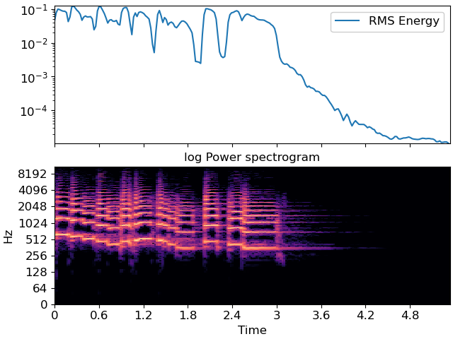
Or from spectrogram input

>>> S, phase = librosa.magphase(librosa.stft(y))
>>> rms = librosa.feature.rms(S=S)

>>> import matplotlib.pyplot as plt
>>> fig, ax = plt.subplots(nrows=2, sharex=True)
>>> times = librosa.times_like(rms)
>>> ax[0].semilogy(times, rms[0], label='RMS Energy')
>>> ax[0].set(xticks=[])
>>> ax[0].legend()
>>> ax[0].label_outer()
>>> librosa.display.specshow(librosa.amplitude_to_db(S, ref=np.max),
...                          y_axis='log', x_axis='time', ax=ax[1])
>>> ax[1].set(title='log Power spectrogram')

Use a STFT window of constant ones and no frame centering to get consistent results with the RMS computed from the audio samples y

>>> S = librosa.magphase(librosa.stft(y, window=np.ones, center=False))[0]
>>> librosa.feature.rms(S=S)
>>> plt.show()