Caution

You're reading an old version of this documentation. If you want up-to-date information, please have a look at 0.10.2.

librosa.cqt

librosa.cqt(y, *, sr=22050, hop_length=512, fmin=None, n_bins=84, bins_per_octave=12, tuning=0.0, filter_scale=1, norm=1, sparsity=0.01, window='hann', scale=True, pad_mode='constant', res_type=None, dtype=None)[source]

Compute the constant-Q transform of an audio signal.

This implementation is based on the recursive sub-sampling method described by [1].

Parameters:

ynp.ndarray [shape=(…, n)]

audio time series. Multi-channel is supported.

srnumber > 0 [scalar]

sampling rate of y

hop_lengthint > 0 [scalar]

number of samples between successive CQT columns.

fminfloat > 0 [scalar]

Minimum frequency. Defaults to C1 ~= 32.70 Hz

n_binsint > 0 [scalar]

Number of frequency bins, starting at fmin

bins_per_octaveint > 0 [scalar]

Number of bins per octave

tuningNone or float

Tuning offset in fractions of a bin.

If None, tuning will be automatically estimated from the signal.

The minimum frequency of the resulting CQT will be modified to fmin * 2**(tuning / bins_per_octave).

filter_scalefloat > 0

Filter scale factor. Small values (<1) use shorter windows for improved time resolution.

norm{inf, -inf, 0, float > 0}

Type of norm to use for basis function normalization. See librosa.util.normalize.

sparsityfloat in [0, 1)

Sparsify the CQT basis by discarding up to sparsity fraction of the energy in each basis.

Set sparsity=0 to disable sparsification.

windowstr, tuple, number, or function

Window specification for the basis filters. See filters.get_window for details.

scalebool

If True, scale the CQT response by square-root the length of each channel’s filter. This is analogous to norm='ortho' in FFT.

If False, do not scale the CQT. This is analogous to norm=None in FFT.

pad_modestring

Padding mode for centered frame analysis.

See also: librosa.stft and numpy.pad.

res_typestring [optional]

The resampling mode for recursive downsampling.

By default, cqt will adaptively select a resampling mode which trades off accuracy at high frequencies for efficiency at low frequencies.

You can override this by specifying a resampling mode as supported by librosa.resample. For example, res_type='fft' will use a high-quality, but potentially slow FFT-based down-sampling, while res_type='polyphase' will use a fast, but potentially inaccurate down-sampling.

dtypenp.dtype

The (complex) data type of the output array. By default, this is inferred to match the numerical precision of the input signal.

Returns:

CQTnp.ndarray [shape=(…, n_bins, t)]: Constant-Q value each frequency at each time.

See also

vqt
librosa.resample
librosa.util.normalize

Notes

This function caches at level 20.

Examples

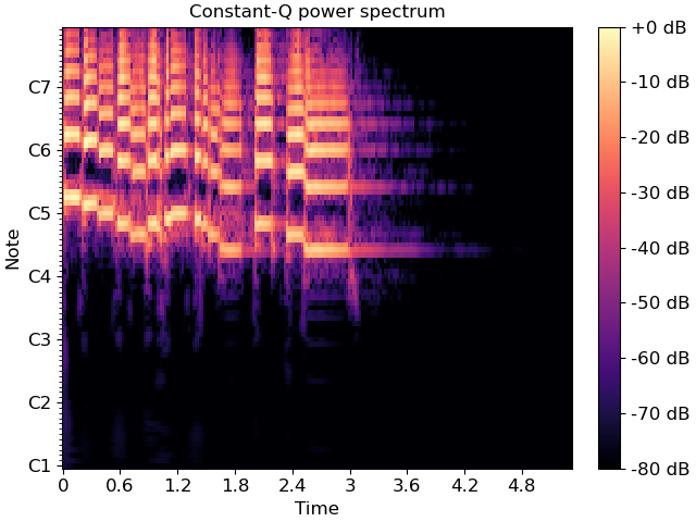
Generate and plot a constant-Q power spectrum

>>> import matplotlib.pyplot as plt
>>> y, sr = librosa.load(librosa.ex('trumpet'))
>>> C = np.abs(librosa.cqt(y, sr=sr))
>>> fig, ax = plt.subplots()
>>> img = librosa.display.specshow(librosa.amplitude_to_db(C, ref=np.max),
...                                sr=sr, x_axis='time', y_axis='cqt_note', ax=ax)
>>> ax.set_title('Constant-Q power spectrum')
>>> fig.colorbar(img, ax=ax, format="%+2.0f dB")

Limit the frequency range

>>> C = np.abs(librosa.cqt(y, sr=sr, fmin=librosa.note_to_hz('C2'),
...                 n_bins=60))
>>> C
array([[6.830e-04, 6.361e-04, ..., 7.362e-09, 9.102e-09],
       [5.366e-04, 4.818e-04, ..., 8.953e-09, 1.067e-08],
       ...,
       [4.288e-02, 4.580e-01, ..., 1.529e-05, 5.572e-06],
       [2.965e-03, 1.508e-01, ..., 8.965e-06, 1.455e-05]])

Using a higher frequency resolution

>>> C = np.abs(librosa.cqt(y, sr=sr, fmin=librosa.note_to_hz('C2'),
...                 n_bins=60 * 2, bins_per_octave=12 * 2))
>>> C
array([[5.468e-04, 5.382e-04, ..., 5.911e-09, 6.105e-09],
       [4.118e-04, 4.014e-04, ..., 7.788e-09, 8.160e-09],
       ...,
       [2.780e-03, 1.424e-01, ..., 4.225e-06, 2.388e-05],
       [5.147e-02, 6.959e-02, ..., 1.694e-05, 5.811e-06]])