librosa.feature.tempogram

librosa.feature.tempogram(*, y=None, sr=22050, onset_envelope=None, hop_length=512, win_length=384, center=True, window='hann', norm=inf)

Compute the tempogram: local autocorrelation of the onset strength envelope. [1]

[1]

Grosche, Peter, Meinard Müller, and Frank Kurth. “Cyclic tempogram - A mid-level tempo representation for music signals.” ICASSP, 2010.

Parameters:

ynp.ndarray [shape=(…, n)] or None

Audio time series. Multi-channel is supported.

srnumber > 0 [scalar]

sampling rate of y

onset_envelopenp.ndarray [shape=(…, n) or (…, m, n)] or None

Optional pre-computed onset strength envelope as provided by librosa.onset.onset_strength.

If multi-dimensional, tempograms are computed independently for each band (first dimension).

hop_lengthint > 0

number of audio samples between successive onset measurements

win_lengthint > 0

length of the onset autocorrelation window (in frames/onset measurements) The default settings (384) corresponds to 384 * hop_length / sr ~= 8.9s.

centerbool

If True, onset autocorrelation windows are centered. If False, windows are left-aligned.

windowstring, function, number, tuple, or np.ndarray [shape=(win_length,)]

A window specification as in stft.

norm{np.inf, -np.inf, 0, float > 0, None}

Normalization mode. Set to None to disable normalization.

Returns:

tempogramnp.ndarray [shape=(…, win_length, n)]

Localized autocorrelation of the onset strength envelope.

If given multi-band input (onset_envelope.shape==(m,n)) then tempogram[i] is the tempogram of onset_envelope[i].

Raises:

ParameterError

if neither y nor onset_envelope are provided

if win_length < 1

See also

fourier_tempogram

librosa.onset.onset_strength

librosa.util.normalize

librosa.stft

Examples

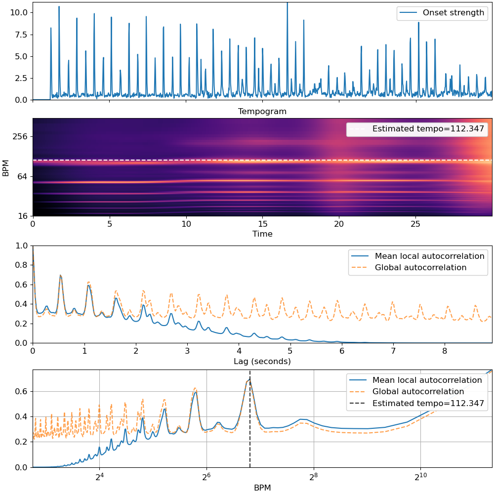
>>> # Compute local onset autocorrelation
>>> y, sr = librosa.load(librosa.ex('nutcracker'), duration=30)
>>> hop_length = 512
>>> oenv = librosa.onset.onset_strength(y=y, sr=sr, hop_length=hop_length)
>>> tempogram = librosa.feature.tempogram(onset_envelope=oenv, sr=sr,
...                                       hop_length=hop_length)
>>> # Compute global onset autocorrelation
>>> ac_global = librosa.autocorrelate(oenv, max_size=tempogram.shape[0])
>>> ac_global = librosa.util.normalize(ac_global)
>>> # Estimate the global tempo for display purposes
>>> tempo = librosa.feature.tempo(onset_envelope=oenv, sr=sr,
...                               hop_length=hop_length)[0]

>>> import matplotlib.pyplot as plt
>>> fig, ax = plt.subplots(nrows=4, figsize=(10, 10))
>>> times = librosa.times_like(oenv, sr=sr, hop_length=hop_length)
>>> ax[0].plot(times, oenv, label='Onset strength')
>>> ax[0].label_outer()
>>> ax[0].legend(frameon=True)
>>> librosa.display.specshow(tempogram, sr=sr, hop_length=hop_length,
>>>                          x_axis='time', y_axis='tempo', cmap='magma',
...                          ax=ax[1])
>>> ax[1].axhline(tempo, color='w', linestyle='--', alpha=1,
...             label='Estimated tempo={:g}'.format(tempo))
>>> ax[1].legend(loc='upper right')
>>> ax[1].set(title='Tempogram')
>>> x = np.linspace(0, tempogram.shape[0] * float(hop_length) / sr,
...                 num=tempogram.shape[0])
>>> ax[2].plot(x, np.mean(tempogram, axis=1), label='Mean local autocorrelation')
>>> ax[2].plot(x, ac_global, '--', alpha=0.75, label='Global autocorrelation')
>>> ax[2].set(xlabel='Lag (seconds)')
>>> ax[2].legend(frameon=True)
>>> freqs = librosa.tempo_frequencies(tempogram.shape[0], hop_length=hop_length, sr=sr)
>>> ax[3].semilogx(freqs[1:], np.mean(tempogram[1:], axis=1),
...              label='Mean local autocorrelation', base=2)
>>> ax[3].semilogx(freqs[1:], ac_global[1:], '--', alpha=0.75,
...              label='Global autocorrelation', base=2)
>>> ax[3].axvline(tempo, color='black', linestyle='--', alpha=.8,
...             label='Estimated tempo={:g}'.format(tempo))
>>> ax[3].legend(frameon=True)
>>> ax[3].set(xlabel='BPM')
>>> ax[3].grid(True)