Caution

You're reading the documentation for a development version. For the latest released version, please have a look at 0.10.2.

Efficient patch generation

This notebook demonstrates how to efficiently generate fixed-duration excerpts of a signal using librosa.util.frame. This can be helpful in machine learning applications where a model may expect inputs of a certain size during training, but your data may be of arbitrary and variable length.

Aside from being a convenient helper method for patch sampling, the librosa.util.frame function can do this efficiently by avoiding memory copies. The patch array produced below is a view of the original data array, not a copy.

import numpy as np
import matplotlib.pyplot as plt
import matplotlib.animation as animation
import librosa

Load an example clip

y, sr = librosa.load(librosa.ex('libri1'))

Compute a log-scaled Mel spectrogram

melspec = librosa.power_to_db(librosa.feature.melspectrogram(y=y, sr=sr),
                              ref=np.max)

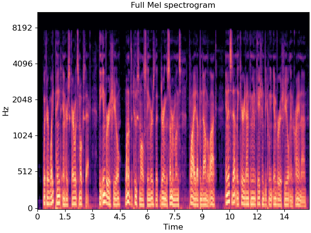
The resulting spectrogram has a number of frames that depends on the length of the input signal y:

print(f"Mel spectrogram shape: {melspec.shape}")

Mel spectrogram shape: (128, 640)

fig, ax = plt.subplots()
librosa.display.specshow(melspec, x_axis='time', y_axis='mel', ax=ax)
ax.set(title='Full Mel spectrogram')

We can use librosa.util.frame to carve melspec into patches of fixed duration.

In this case, we’ll make ~5-second patches separated by approximately 1/10 second each.

frame_length = librosa.time_to_frames(5.0)
hop_length = librosa.time_to_frames(0.10)
print(f"Frame length={frame_length}, hop length={hop_length}")

Frame length=215, hop length=4

patches = librosa.util.frame(melspec,
                             frame_length=frame_length,
                             hop_length=hop_length)

The resulting patches array is now three-dimensional, with axes corresponding to [frequency, time, patch index]

print(f"Patch array shape: {patches.shape}")

Patch array shape: (128, 215, 107)

So patches[..., 0] is the first 1-second patch, patches[..., 1] is the second 1-second patch, and so on. All patches will have the same shape.

Unlike the framing operation used by spectrogram functions, these patches are not centered; they are left-aligned. This means that the first patch, patches[..., 0] corresponds to the original data melspec[..., 0:frame_length]. The second patch patches[..., 1] corresponds to data melspec[..., hop_length:hop_length+frame_length], the third patch patches[..., 2] corresponds to melspec[..., 2*hop_length:2*hop_length+frame_length], etc.

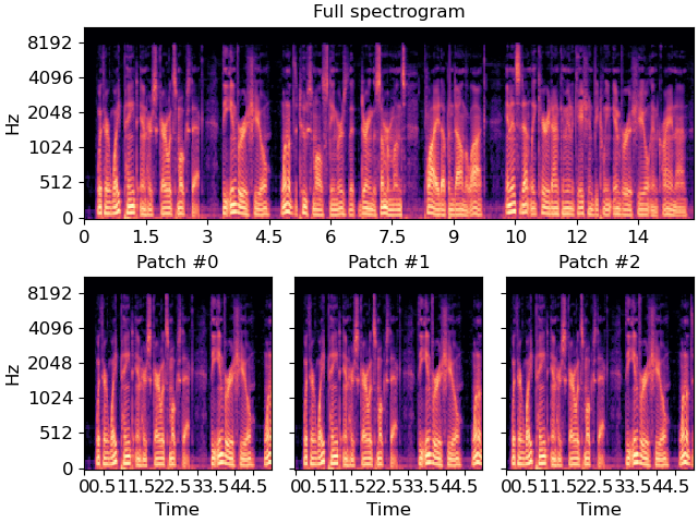
The figure below illustrates the first three patches. Because the overlap (1/10) is small relative to the patch length (5), these patches have substantial overlap and contain mostly the same content but at different time offsets.

fig, ax = plt.subplot_mosaic([list("AAA"), list("012")])

librosa.display.specshow(melspec, x_axis='time', y_axis='mel', ax=ax["A"])
ax["A"].set(title='Full spectrogram', xlabel=None)

for index in [0, 1, 2]:
    librosa.display.specshow(patches[..., index],
                             x_axis='time', y_axis='mel',
                             ax=ax[str(index)])
    ax[str(index)].set(title=f"Patch #{index}")
    ax[str(index)].label_outer()

The animation below illustrates each patch in approximate real time.

# We'll plot the first patch to create the display object,
# then animate the rest.

# sphinx_gallery_thumbnail_number = 2

fig, ax = plt.subplots()
mesh = librosa.display.specshow(patches[..., 0], x_axis='time',
                                y_axis='mel', ax=ax)


# This helper function is used to render each frame of the animation
# Updating the mesh object is much more efficient than rendering an
# entirely new spectrogram for each frame!
#
# Note that the "time" axis of this figure corresponds to the time
# within the patch; not the absolute time in the original signal.
#
def _update(num):
    mesh.set_array(patches[..., num])
    return (mesh,)


ani = animation.FuncAnimation(fig,
                              func=_update,
                              frames=patches.shape[-1],
                              interval=100,  # 100 milliseconds = 1/10 sec
                              blit=True)

Once Loop Reflect