Caution

You're reading the documentation for a development version. For the latest released version, please have a look at 0.10.2.

librosa.decompose.decompose

librosa.decompose.decompose(S, *, n_components=None, transformer=None, sort=False, fit=True, **kwargs)

Decompose a feature matrix.

Given a spectrogram S, produce a decomposition into components and activations such that S ~= components.dot(activations).

By default, this is done with with non-negative matrix factorization (NMF), but any sklearn.decomposition-type object will work.

Parameters:

Snp.ndarray [shape=(…, n_features, n_samples), dtype=float]

The input feature matrix (e.g., magnitude spectrogram)

If the input has multiple channels (leading dimensions), they will be automatically flattened prior to decomposition.

If the input is multi-channel, channels and features are automatically flattened into a single axis before the decomposition. For example, a stereo input S with shape (2, n_features, n_samples) is automatically reshaped to (2 * n_features, n_samples).

n_componentsint > 0 [scalar] or None

number of desired components

if None, then n_features components are used

transformerNone or object

If None, use sklearn.decomposition.NMF

Otherwise, any object with a similar interface to NMF should work. transformer must follow the scikit-learn convention, where input data is (n_samples, n_features).

transformer.fit_transform() will be run on S.T (not S), the return value of which is stored (transposed) as activations

The components will be retrieved as transformer.components_.T:

S ~= np.dot(activations, transformer.components_).T

or equivalently:

S ~= np.dot(transformer.components_.T, activations.T)

sortbool

If True, components are sorted by ascending peak frequency.

Note

If used with transformer, sorting is applied to copies of the decomposition parameters, and not to transformer internal parameters.

Warning

If the input array has more than two dimensions (e.g., if it’s a multi-channel spectrogram), then axis sorting is not supported and a ParameterError exception is raised.

fitbool

If True, components are estimated from the input S.

If False, components are assumed to be pre-computed and stored in transformer, and are not changed.

**kwargsAdditional keyword arguments to the default transformer

sklearn.decomposition.NMF

Returns:

components: np.ndarray [shape=(…, n_features, n_components)]

matrix of components (basis elements).

activations: np.ndarray [shape=(n_components, n_samples)]

transformed matrix/activation matrix

Raises:

ParameterError

if fit is False and no transformer object is provided.

if the input array is multi-channel and sort=True is specified.

See also

sklearn.decomposition

SciKit-Learn matrix decomposition modules

Examples

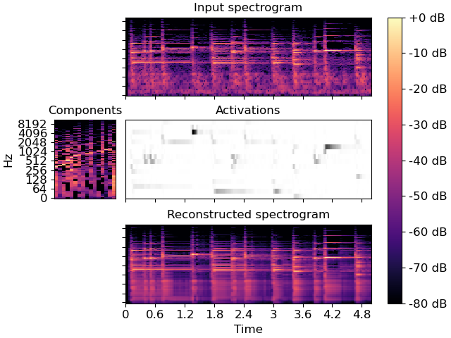
Decompose a magnitude spectrogram into 16 components with NMF

>>> y, sr = librosa.load(librosa.ex('pistachio'), duration=5)
>>> S = np.abs(librosa.stft(y))
>>> comps, acts = librosa.decompose.decompose(S, n_components=16)

Sort components by ascending peak frequency

>>> comps, acts = librosa.decompose.decompose(S, n_components=16,
...                                           sort=True)

Or with sparse dictionary learning

>>> import sklearn.decomposition
>>> T = sklearn.decomposition.MiniBatchDictionaryLearning(n_components=16)
>>> scomps, sacts = librosa.decompose.decompose(S, transformer=T, sort=True)

>>> import matplotlib.pyplot as plt
>>> layout = [list(".AAAA"), list("BCCCC"), list(".DDDD")]
>>> fig, ax = plt.subplot_mosaic(layout, constrained_layout=True)
>>> librosa.display.specshow(librosa.amplitude_to_db(S, ref=np.max),
...                          y_axis='log', x_axis='time', ax=ax['A'])
>>> ax['A'].set(title='Input spectrogram')
>>> ax['A'].label_outer()
>>> librosa.display.specshow(librosa.amplitude_to_db(comps,
>>>                                                  ref=np.max),
>>>                          y_axis='log', ax=ax['B'])
>>> ax['B'].set(title='Components')
>>> ax['B'].label_outer()
>>> ax['B'].sharey(ax['A'])
>>> librosa.display.specshow(acts, x_axis='time', ax=ax['C'], cmap='gray_r')
>>> ax['C'].set(ylabel='Components', title='Activations')
>>> ax['C'].sharex(ax['A'])
>>> ax['C'].label_outer()
>>> S_approx = comps.dot(acts)
>>> img = librosa.display.specshow(librosa.amplitude_to_db(S_approx,
>>>                                                        ref=np.max),
>>>                                y_axis='log', x_axis='time', ax=ax['D'])
>>> ax['D'].set(title='Reconstructed spectrogram')
>>> ax['D'].sharex(ax['A'])
>>> ax['D'].sharey(ax['A'])
>>> ax['D'].label_outer()
>>> fig.colorbar(img, ax=list(ax.values()), format="%+2.f dB")