Caution

You're reading the documentation for a development version. For the latest released version, please have a look at 0.10.2.

librosa.feature.spectral_centroid

librosa.feature.spectral_centroid(*, y=None, sr=22050, S=None, n_fft=2048, hop_length=512, freq=None, win_length=None, window='hann', center=True, pad_mode='constant')

Compute the spectral centroid.

Each frame of a magnitude spectrogram is normalized and treated as a distribution over frequency bins, from which the mean (centroid) is extracted per frame.

More precisely, the centroid at frame t is defined as [1]:

centroid[t] = sum_k S[k, t] * freq[k] / (sum_j S[j, t])

where S is a magnitude spectrogram, and freq is the array of frequencies (e.g., FFT frequencies in Hz) of the rows of S.

[1]

Klapuri, A., & Davy, M. (Eds.). (2007). Signal processing methods for music transcription, chapter 5. Springer Science & Business Media.

Parameters:

ynp.ndarray [shape=(…, n,)] or None

audio time series. Multi-channel is supported.

srnumber > 0 [scalar]

audio sampling rate of y

Snp.ndarray [shape=(…, d, t)] or None

(optional) spectrogram magnitude

n_fftint > 0 [scalar]

FFT window size

hop_lengthint > 0 [scalar]

hop length for STFT. See librosa.stft for details.

freqNone or np.ndarray [shape=(d,) or shape=(d, t)]

Center frequencies for spectrogram bins. If None, then FFT bin center frequencies are used. Otherwise, it can be a single array of d center frequencies, or a matrix of center frequencies as constructed by librosa.reassigned_spectrogram

win_lengthint <= n_fft [scalar]

Each frame of audio is windowed by window(). The window will be of length win_length and then padded with zeros to match n_fft. If unspecified, defaults to win_length = n_fft.

windowstring, tuple, number, function, or np.ndarray [shape=(n_fft,)]

• a window specification (string, tuple, or number); see scipy.signal.get_window

• a window function, such as scipy.signal.windows.hann

• a vector or array of length n_fft

centerboolean

• If True, the signal y is padded so that frame t is centered at y[t * hop_length].

• If False, then frame t begins at y[t * hop_length]

pad_modestring

If center=True, the padding mode to use at the edges of the signal. By default, STFT uses zero padding.

Returns:

centroidnp.ndarray [shape=(…, 1, t)]

centroid frequencies

See also

librosa.stft

Short-time Fourier Transform

librosa.reassigned_spectrogram

Time-frequency reassigned spectrogram

Examples

From time-series input:

>>> y, sr = librosa.load(librosa.ex('trumpet'))
>>> cent = librosa.feature.spectral_centroid(y=y, sr=sr)
>>> cent
array([[1768.888, 1921.774, ..., 5663.477, 5813.683]])

From spectrogram input:

>>> S, phase = librosa.magphase(librosa.stft(y=y))
>>> librosa.feature.spectral_centroid(S=S)
array([[1768.888, 1921.774, ..., 5663.477, 5813.683]])

Using variable bin center frequencies:

>>> freqs, times, D = librosa.reassigned_spectrogram(y, fill_nan=True)
>>> librosa.feature.spectral_centroid(S=np.abs(D), freq=freqs)
array([[1768.838, 1921.801, ..., 5663.513, 5813.747]])

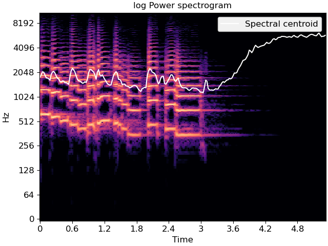
Plot the result

>>> import matplotlib.pyplot as plt
>>> times = librosa.times_like(cent)
>>> fig, ax = plt.subplots()
>>> librosa.display.specshow(librosa.amplitude_to_db(S, ref=np.max),
...                          y_axis='log', x_axis='time', ax=ax)
>>> ax.plot(times, cent.T, label='Spectral centroid', color='w')
>>> ax.legend(loc='upper right')
>>> ax.set(title='log Power spectrogram')