Caution

You're reading an old version of this documentation. If you want up-to-date information, please have a look at 0.9.1.

librosa.feature.fourier_tempogram

librosa.feature.fourier_tempogram(y=None, sr=22050, onset_envelope=None, hop_length=512, win_length=384, center=True, window='hann')

Compute the Fourier tempogram: the short-time Fourier transform of the onset strength envelope. [1]

1

Grosche, Peter, Meinard Müller, and Frank Kurth. “Cyclic tempogram - A mid-level tempo representation for music signals.” ICASSP, 2010.

Parameters

ynp.ndarray [shape=(n,)] or None

Audio time series.

srnumber > 0 [scalar]

sampling rate of y

onset_envelopenp.ndarray [shape=(n,)] or None

Optional pre-computed onset strength envelope as provided by onset.onset_strength.

hop_lengthint > 0

number of audio samples between successive onset measurements

win_lengthint > 0

length of the onset window (in frames/onset measurements) The default settings (384) corresponds to 384 * hop_length / sr ~= 8.9s.

centerbool

If True, onset windows are centered. If False, windows are left-aligned.

windowstring, function, number, tuple, or np.ndarray [shape=(win_length,)]

A window specification as in core.stft.

Returns

tempogramnp.ndarray [shape=(win_length // 2 + 1, n)]

Complex short-time Fourier transform of the onset envelope.

Raises

ParameterError

if neither y nor onset_envelope are provided

if win_length < 1

See also

tempogram

librosa.onset.onset_strength

librosa.util.normalize

librosa.core.stft

Examples

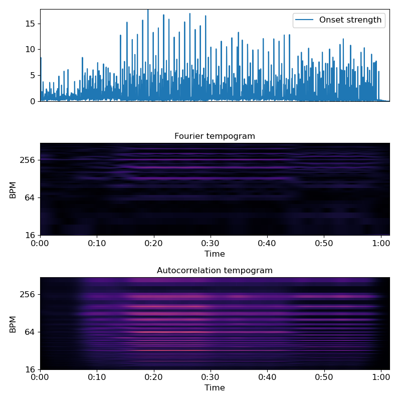
>>> # Compute local onset autocorrelation
>>> y, sr = librosa.load(librosa.util.example_audio_file())
>>> hop_length = 512
>>> oenv = librosa.onset.onset_strength(y=y, sr=sr, hop_length=hop_length)
>>> tempogram = librosa.feature.fourier_tempogram(onset_envelope=oenv, sr=sr,
...                                               hop_length=hop_length)
>>> # Compute the auto-correlation tempogram, unnormalized to make comparison easier
>>> ac_tempogram = librosa.feature.tempogram(onset_envelope=oenv, sr=sr,
...                                          hop_length=hop_length, norm=None)

>>> import matplotlib.pyplot as plt
>>> plt.figure(figsize=(8, 8))
>>> plt.subplot(3, 1, 1)
>>> plt.plot(oenv, label='Onset strength')
>>> plt.xticks([])
>>> plt.legend(frameon=True)
>>> plt.axis('tight')
>>> plt.subplot(3, 1, 2)
>>> librosa.display.specshow(np.abs(tempogram), sr=sr, hop_length=hop_length,
>>>                          x_axis='time', y_axis='fourier_tempo', cmap='magma')
>>> plt.title('Fourier tempogram')
>>> plt.subplot(3, 1, 3)
>>> librosa.display.specshow(ac_tempogram, sr=sr, hop_length=hop_length,
>>>                          x_axis='time', y_axis='tempo', cmap='magma')
>>> plt.title('Autocorrelation tempogram')
>>> plt.tight_layout()
>>> plt.show()