Caution
You're reading an old version of this documentation. If you want up-to-date information, please have a look at 0.9.1.
librosa.core.stft
- librosa.core.stft(y, n_fft=2048, hop_length=None, win_length=None, window='hann', center=True, dtype=<class 'numpy.complex64'>, pad_mode='reflect')[source]
Short-time Fourier transform (STFT). [1] (chapter 2)
The STFT represents a signal in the time-frequency domain by computing discrete Fourier transforms (DFT) over short overlapping windows.
This function returns a complex-valued matrix D such that
np.abs(D[f, t]) is the magnitude of frequency bin f at frame t, and
np.angle(D[f, t]) is the phase of frequency bin f at frame t.
The integers t and f can be converted to physical units by means of the utility functions frames_to_sample and
fft_frequencies.- 1
Müller. “Fundamentals of Music Processing.” Springer, 2015
- Parameters
- ynp.ndarray [shape=(n,)], real-valued
input signal
- n_fftint > 0 [scalar]
length of the windowed signal after padding with zeros. The number of rows in the STFT matrix D is (1 + n_fft/2). The default value, n_fft=2048 samples, corresponds to a physical duration of 93 milliseconds at a sample rate of 22050 Hz, i.e. the default sample rate in librosa. This value is well adapted for music signals. However, in speech processing, the recommended value is 512, corresponding to 23 milliseconds at a sample rate of 22050 Hz. In any case, we recommend setting n_fft to a power of two for optimizing the speed of the fast Fourier transform (FFT) algorithm.
- hop_lengthint > 0 [scalar]
number of audio samples between adjacent STFT columns.
Smaller values increase the number of columns in D without affecting the frequency resolution of the STFT.
If unspecified, defaults to win_length / 4 (see below).
- win_lengthint <= n_fft [scalar]
Each frame of audio is windowed by window() of length win_length and then padded with zeros to match n_fft.
Smaller values improve the temporal resolution of the STFT (i.e. the ability to discriminate impulses that are closely spaced in time) at the expense of frequency resolution (i.e. the ability to discriminate pure tones that are closely spaced in frequency). This effect is known as the time-frequency localization tradeoff and needs to be adjusted according to the properties of the input signal y.
If unspecified, defaults to
win_length = n_fft.- windowstring, tuple, number, function, or np.ndarray [shape=(n_fft,)]
Either:
a window specification (string, tuple, or number); see
scipy.signal.get_windowa window function, such as
scipy.signal.hanninga vector or array of length n_fft
Defaults to a raised cosine window (“hann”), which is adequate for most applications in audio signal processing.
- centerboolean
If True, the signal y is padded so that frame D[:, t] is centered at y[t * hop_length].
If False, then D[:, t] begins at y[t * hop_length].
Defaults to True, which simplifies the alignment of D onto a time grid by means of
librosa.core.frames_to_samples. Note, however, that center must be set to False when analyzing signals withlibrosa.stream.- dtypenumeric type
Complex numeric type for D. Default is single-precision floating-point complex (np.complex64).
- pad_modestring or function
If center=True, this argument is passed to np.pad for padding the edges of the signal y. By default (pad_mode=”reflect”), y is padded on both sides with its own reflection, mirrored around its first and last sample respectively. If center=False, this argument is ignored.
- Returns
- Dnp.ndarray [shape=(1 + n_fft/2, n_frames), dtype=dtype]
Complex-valued matrix of short-term Fourier transform coefficients.
See also
istftInverse STFT
reassigned_spectrogramTime-frequency reassigned spectrogram
Notes
This function caches at level 20.
Examples
>>> y, sr = librosa.load(librosa.util.example_audio_file())
>>> D = np.abs(librosa.stft(y))
>>> D
array([[2.58028018e-03, 4.32422794e-02, 6.61255598e-01, ...,
        6.82710262e-04, 2.51654536e-04, 7.23036574e-05],
       [2.49403086e-03, 5.15930466e-02, 6.00107312e-01, ...,
        3.48026224e-04, 2.35853557e-04, 7.54836728e-05],
       [7.82410789e-04, 1.05394892e-01, 4.37517226e-01, ...,
        6.29352580e-04, 3.38571583e-04, 8.38094638e-05],
       ...,
       [9.48568513e-08, 4.74725084e-07, 1.50052492e-05, ...,
        1.85637656e-08, 2.89708542e-08, 5.74304337e-09],
       [1.25165826e-07, 8.58259284e-07, 1.11157215e-05, ...,
        3.49099771e-08, 3.11740926e-08, 5.29926236e-09],
       [1.70630571e-07, 8.92518756e-07, 1.23656537e-05, ...,
        5.33256745e-08, 3.33264900e-08, 5.13272980e-09]], dtype=float32)
Use left-aligned frames, instead of centered frames
>>> D_left = np.abs(librosa.stft(y, center=False))
Use a shorter hop length
>>> D_short = np.abs(librosa.stft(y, hop_length=64))
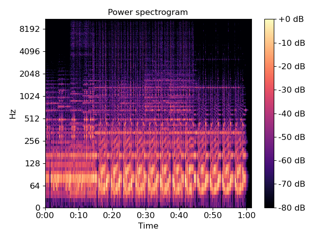
Display a spectrogram
>>> import matplotlib.pyplot as plt
>>> librosa.display.specshow(librosa.amplitude_to_db(D,
...                                                  ref=np.max),
...                          y_axis='log', x_axis='time')
>>> plt.title('Power spectrogram')
>>> plt.colorbar(format='%+2.0f dB')
>>> plt.tight_layout()
>>> plt.show()
