Caution

You're reading the documentation for a development version. For the latest released version, please have a look at 0.11.0.

librosa.feature.metrogram

librosa.feature.metrogram(*, tg, freqs, factors=None, aggregate=<function sum>, kind='linear', fill_value=0)

Metrogram Transform. [1]

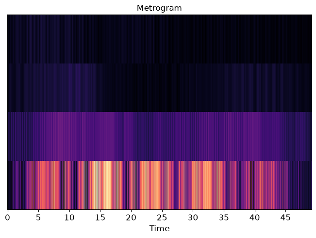
This function summarizes the presence of rhythmic ratios in a tempogram. For example, a tempogram with two simultaneous energy peaks at 90BPM and 30BPM would have a strong presence of the 1/3 ratio. This makes it possible to perform meter estimation by finding the ratio between the beat’s and downbeat’s frequency.

By default, the factors used here are as specified by [2].

Index	Factor	Time Signature
0	1/3	3/4
1	1/4	4/4
2	1/5	5/4
3	1/7	7/4

[1]

Cozens, James, and Simon Godsill. “Dynamic Time Signature Recognition, Tempo Inference, and Beat Tracking Through the Metrogram Transform.” In IEEE Open Journal of Signal Processing, pp. 1–9, 2023.

[2]

Abimbola, Jeremiah, Daniel Kostrzewa, and Paweł Kasprowski. “METER2800: A novel dataset for music time signature detection.” In Data in Brief, vol. 51, 109736, 2023.

Parameters:

tgnp.ndarray

Pre-computed tempogram.

freqsnp.ndarray

Frequencies (in BPM) of the tempogram axis.

factorsnp.ndarray

Metric ratios to estimate. If not provided, the default factors are 1/3, 1/4, 1/5, and 1/7.

aggregatecallable [optional]

Aggregation function to collapse the tempo axis for each ratio at each point in time. Defaults to np.sum.

kindstr

Interpolation method used on the tempo axis.

fill_valuefloat

The value to fill when extrapolating beyond the observed tempo range.

Returns:

metrogramnp.ndarray

The metrogram transform for the specified factors. If aggregate is set to None, the ratios for all individual tempo bins are returned.

See also

tempogram

tempogram_ratio

Examples

>>> import numpy as np
>>> import matplotlib.pyplot as plt
>>> import librosa
>>> y, sr = librosa.loadx("sweetwaltz")
>>> # extend the window, to capture the slower downbeat pulses
>>> win_length = 384 * 4
>>> fourier_tempogram = librosa.feature.fourier_tempogram(y=y, win_length=win_length)
>>> fourier_freqs = librosa.fourier_tempo_frequencies(win_length=win_length)
>>> ac_tempogram = librosa.feature.tempogram(y=y, win_length=win_length)
>>> ac_freqs = librosa.tempo_frequencies(ac_tempogram.shape[-2])
>>> # combine Fourier and AC tempo grid (alternatively, you may use either one)
>>> # we remove np.inf from ac_freqs to avoid nan results
>>> funt_freqs = np.union1d(fourier_freqs, ac_freqs[1:])
>>> fundamental_tempogram = librosa.util.interp_broadcast(
...     x1=ac_tempogram,
...     x1_pos=ac_freqs,
...     x2=fourier_tempogram[..., :-1],  # both tempograms must be of equal length along time
...     x2_pos=fourier_freqs,
...     interp_pos=funt_freqs,
... )
>>> metrogram = librosa.feature.metrogram(tg=fundamental_tempogram, freqs=funt_freqs)
>>> fig, ax = plt.subplots()
>>> librosa.display.specshow(np.abs(metrogram), x_axis="time", ax=ax)
>>> ax.set(title="Metrogram")