Caution

You're reading an old version of this documentation. If you want up-to-date information, please have a look at 0.9.1.

Enhanced chroma and chroma variants

This notebook demonstrates a variety of techniques for enhancing chroma features and also, introduces chroma variants implemented in librosa.

Enhanced chroma

Beyond the default parameter settings of librosa’s chroma functions, we apply the following enhancements:

1. Over-sampling the frequency axis to reduce sensitivity to tuning deviations

2. Harmonic-percussive-residual source separation to eliminate transients.

3. Nearest-neighbor smoothing to eliminate passing tones and sparse noise. This is inspired by the recurrence-based smoothing technique of Cho and Bello, 2011.

4. Local median filtering to suppress remaining discontinuities.

# Code source: Brian McFee
# License: ISC
# sphinx_gallery_thumbnail_number = 6

from __future__ import print_function
import numpy as np
import scipy
import matplotlib.pyplot as plt

import librosa
import librosa.display

We’ll use a track that has harmonic, melodic, and percussive elements

y, sr = librosa.load('audio/Karissa_Hobbs_-_09_-_Lets_Go_Fishin.mp3')

Out:

/tmp/tmpfl4ra6qp/b0064fe7dbe8048b1d4148e61a568b6fe3fca91b/librosa/core/audio.py:161: UserWarning: PySoundFile failed. Trying audioread instead.
  warnings.warn('PySoundFile failed. Trying audioread instead.')

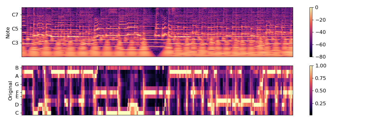
First, let’s plot the original chroma

chroma_orig = librosa.feature.chroma_cqt(y=y, sr=sr)

# For display purposes, let's zoom in on a 15-second chunk from the middle of the song
idx = tuple([slice(None), slice(*list(librosa.time_to_frames([45, 60])))])

# And for comparison, we'll show the CQT matrix as well.
C = np.abs(librosa.cqt(y=y, sr=sr, bins_per_octave=12*3, n_bins=7*12*3))


plt.figure(figsize=(12, 4))
plt.subplot(2, 1, 1)
librosa.display.specshow(librosa.amplitude_to_db(C, ref=np.max)[idx],
                         y_axis='cqt_note', bins_per_octave=12*3)
plt.colorbar()
plt.subplot(2, 1, 2)
librosa.display.specshow(chroma_orig[idx], y_axis='chroma')
plt.colorbar()
plt.ylabel('Original')
plt.tight_layout()

Out:

/tmp/tmpfl4ra6qp/b0064fe7dbe8048b1d4148e61a568b6fe3fca91b/librosa/display.py:862: MatplotlibDeprecationWarning: The 'basey' parameter of __init__() has been renamed 'base' since Matplotlib 3.3; support for the old name will be dropped two minor releases later.
  scaler(mode, **kwargs)

We can correct for minor tuning deviations by using 3 CQT bins per semi-tone, instead of one

chroma_os = librosa.feature.chroma_cqt(y=y, sr=sr, bins_per_octave=12*3)


plt.figure(figsize=(12, 4))

plt.subplot(2, 1, 1)
librosa.display.specshow(chroma_orig[idx], y_axis='chroma')
plt.colorbar()
plt.ylabel('Original')


plt.subplot(2, 1, 2)
librosa.display.specshow(chroma_os[idx], y_axis='chroma', x_axis='time')
plt.colorbar()
plt.ylabel('3x-over')
plt.tight_layout()

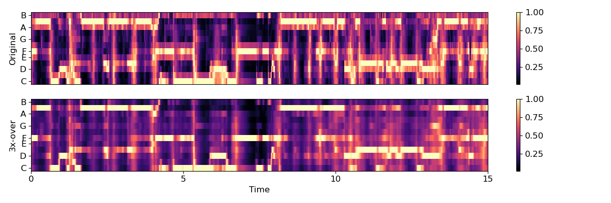
That cleaned up some rough edges, but we can do better by isolating the harmonic component. We’ll use a large margin for separating harmonics from percussives

y_harm = librosa.effects.harmonic(y=y, margin=8)
chroma_os_harm = librosa.feature.chroma_cqt(y=y_harm, sr=sr, bins_per_octave=12*3)


plt.figure(figsize=(12, 4))

plt.subplot(2, 1, 1)
librosa.display.specshow(chroma_os[idx], y_axis='chroma')
plt.colorbar()
plt.ylabel('3x-over')

plt.subplot(2, 1, 2)
librosa.display.specshow(chroma_os_harm[idx], y_axis='chroma', x_axis='time')
plt.colorbar()
plt.ylabel('Harmonic')
plt.tight_layout()

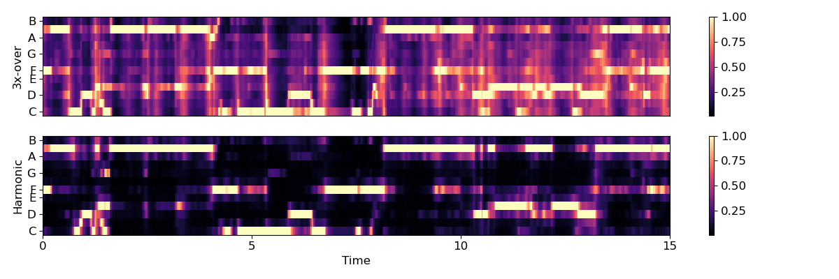
There’s still some noise in there though. We can clean it up using non-local filtering. This effectively removes any sparse additive noise from the features.

chroma_filter = np.minimum(chroma_os_harm,
                           librosa.decompose.nn_filter(chroma_os_harm,
                                                       aggregate=np.median,
                                                       metric='cosine'))


plt.figure(figsize=(12, 4))

plt.subplot(2, 1, 1)
librosa.display.specshow(chroma_os_harm[idx], y_axis='chroma')
plt.colorbar()
plt.ylabel('Harmonic')

plt.subplot(2, 1, 2)
librosa.display.specshow(chroma_filter[idx], y_axis='chroma', x_axis='time')
plt.colorbar()
plt.ylabel('Non-local')
plt.tight_layout()

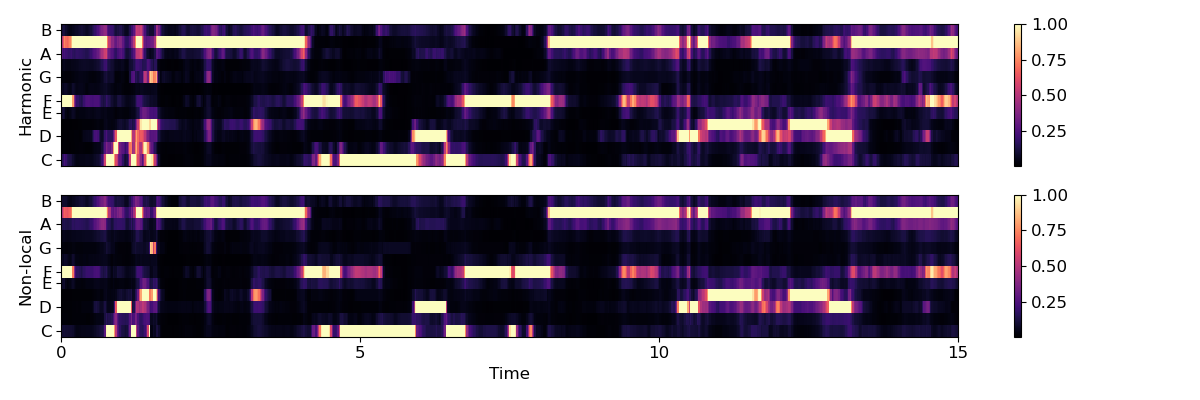
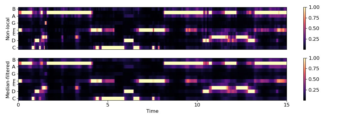
Local discontinuities and transients can be suppressed by using a horizontal median filter.

chroma_smooth = scipy.ndimage.median_filter(chroma_filter, size=(1, 9))


plt.figure(figsize=(12, 4))

plt.subplot(2, 1, 1)
librosa.display.specshow(chroma_filter[idx], y_axis='chroma')
plt.colorbar()
plt.ylabel('Non-local')

plt.subplot(2, 1, 2)
librosa.display.specshow(chroma_smooth[idx], y_axis='chroma', x_axis='time')
plt.colorbar()
plt.ylabel('Median-filtered')
plt.tight_layout()

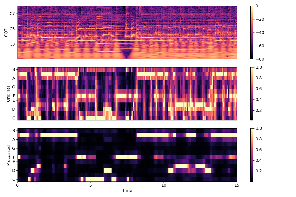
A final comparison between the CQT, original chromagram and the result of our filtering.

plt.figure(figsize=(12, 8))
plt.subplot(3, 1, 1)
librosa.display.specshow(librosa.amplitude_to_db(C, ref=np.max)[idx],
                         y_axis='cqt_note', bins_per_octave=12*3)
plt.colorbar()
plt.ylabel('CQT')
plt.subplot(3, 1, 2)
librosa.display.specshow(chroma_orig[idx], y_axis='chroma')
plt.ylabel('Original')
plt.colorbar()
plt.subplot(3, 1, 3)
librosa.display.specshow(chroma_smooth[idx], y_axis='chroma', x_axis='time')
plt.ylabel('Processed')
plt.colorbar()
plt.tight_layout()
plt.show()

Out:

/tmp/tmpfl4ra6qp/b0064fe7dbe8048b1d4148e61a568b6fe3fca91b/librosa/display.py:862: MatplotlibDeprecationWarning: The 'basey' parameter of __init__() has been renamed 'base' since Matplotlib 3.3; support for the old name will be dropped two minor releases later.
  scaler(mode, **kwargs)

Chroma variants

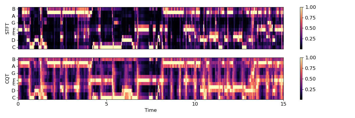
There are three chroma variants implemented in librosa: chroma_stft, chroma_cqt, and chroma_cens. chroma_stft and chroma_cqt are two alternative ways of plotting chroma.

chroma_stft performs short-time fourier transform of an audio input and maps each STFT bin to chroma, while chroma_cqt uses constant-Q transform and maps each cq-bin to chroma.

A comparison between the STFT and the CQT methods for chromagram.

chromagram_stft = librosa.feature.chroma_stft(y=y, sr=sr)
chromagram_cqt = librosa.feature.chroma_cqt(y=y, sr=sr)


plt.figure(figsize=(12, 4))

plt.subplot(2, 1, 1)
librosa.display.specshow(chromagram_stft[idx], y_axis='chroma')
plt.colorbar()
plt.ylabel('STFT')

plt.subplot(2, 1, 2)
librosa.display.specshow(chromagram_cqt[idx], y_axis='chroma', x_axis='time')
plt.colorbar()
plt.ylabel('CQT')
plt.tight_layout()

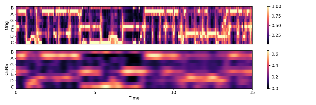
CENS features (chroma_cens) are variants of chroma features introduced in Müller and Ewart, 2011, in which additional post processing steps are performed on the constant-Q chromagram to obtain features that are invariant to dynamics and timbre.

Thus, the CENS features are useful for applications, such as audio matching and retrieval.

Following steps are additional processing done on the chromagram, and are implemented in chroma_cens:

1. L1-Normalization across each chroma vector

2. Quantization of the amplitudes based on “log-like” amplitude thresholds

3. Smoothing with sliding window (optional parameter)

4. Downsampling (not implemented)

A comparison between the original constant-Q chromagram and the CENS features.

chromagram_cens = librosa.feature.chroma_cens(y=y, sr=sr)


plt.figure(figsize=(12, 4))

plt.subplot(2, 1, 1)
librosa.display.specshow(chromagram_cqt[idx], y_axis='chroma')
plt.colorbar()
plt.ylabel('Orig')

plt.subplot(2, 1, 2)
librosa.display.specshow(chromagram_cens[idx], y_axis='chroma', x_axis='time')
plt.colorbar()
plt.ylabel('CENS')
plt.tight_layout()