Caution

You're reading an old version of this documentation. If you want up-to-date information, please have a look at 0.9.1.

librosa.feature.chroma_stft

librosa.feature.chroma_stft(y=None, sr=22050, S=None, norm=inf, n_fft=2048, hop_length=512, win_length=None, window='hann', center=True, pad_mode='reflect', tuning=None, n_chroma=12, **kwargs)

Compute a chromagram from a waveform or power spectrogram.

This implementation is derived from chromagram_E [1]

1

Ellis, Daniel P.W. “Chroma feature analysis and synthesis” 2007/04/21 http://labrosa.ee.columbia.edu/matlab/chroma-ansyn/

Parameters

ynp.ndarray [shape=(n,)] or None

audio time series

srnumber > 0 [scalar]

sampling rate of y

Snp.ndarray [shape=(d, t)] or None

power spectrogram

normfloat or None

Column-wise normalization. See librosa.util.normalize for details.

If None, no normalization is performed.

n_fftint > 0 [scalar]

FFT window size if provided y, sr instead of S

hop_lengthint > 0 [scalar]

hop length if provided y, sr instead of S

win_lengthint <= n_fft [scalar]

Each frame of audio is windowed by window(). The window will be of length win_length and then padded with zeros to match n_fft.

If unspecified, defaults to win_length = n_fft.

windowstring, tuple, number, function, or np.ndarray [shape=(n_fft,)]

• a window specification (string, tuple, or number); see scipy.signal.get_window

• a window function, such as scipy.signal.hanning

• a vector or array of length n_fft

centerboolean

• If True, the signal y is padded so that frame t is centered at y[t * hop_length].

• If False, then frame t begins at y[t * hop_length]

pad_modestring

If center=True, the padding mode to use at the edges of the signal. By default, STFT uses reflection padding.

tuningfloat [scalar] or None.

Deviation from A440 tuning in fractional chroma bins. If None, it is automatically estimated.

n_chromaint > 0 [scalar]

Number of chroma bins to produce (12 by default).

kwargsadditional keyword arguments

Arguments to parameterize chroma filters. See librosa.filters.chroma for details.

Returns

chromagramnp.ndarray [shape=(n_chroma, t)]

Normalized energy for each chroma bin at each frame.

See also

librosa.filters.chroma

Chroma filter bank construction

librosa.util.normalize

Vector normalization

Examples

>>> y, sr = librosa.load(librosa.util.example_audio_file())
>>> librosa.feature.chroma_stft(y=y, sr=sr)
array([[ 0.974,  0.881, ...,  0.925,  1.   ],
       [ 1.   ,  0.841, ...,  0.882,  0.878],
       ...,
       [ 0.658,  0.985, ...,  0.878,  0.764],
       [ 0.969,  0.92 , ...,  0.974,  0.915]])

Use an energy (magnitude) spectrum instead of power spectrogram

>>> S = np.abs(librosa.stft(y))
>>> chroma = librosa.feature.chroma_stft(S=S, sr=sr)
>>> chroma
array([[ 0.884,  0.91 , ...,  0.861,  0.858],
       [ 0.963,  0.785, ...,  0.968,  0.896],
       ...,
       [ 0.871,  1.   , ...,  0.928,  0.829],
       [ 1.   ,  0.982, ...,  0.93 ,  0.878]])

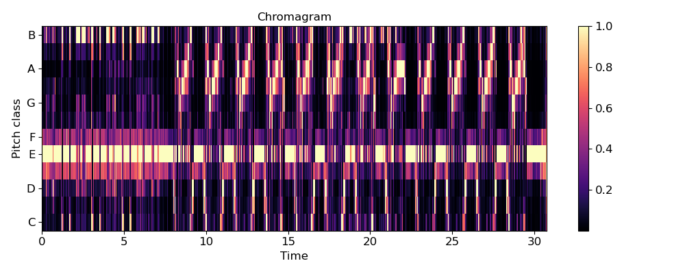
Use a pre-computed power spectrogram with a larger frame

>>> S = np.abs(librosa.stft(y, n_fft=4096))**2
>>> chroma = librosa.feature.chroma_stft(S=S, sr=sr)
>>> chroma
array([[ 0.685,  0.477, ...,  0.961,  0.986],
       [ 0.674,  0.452, ...,  0.952,  0.926],
       ...,
       [ 0.844,  0.575, ...,  0.934,  0.869],
       [ 0.793,  0.663, ...,  0.964,  0.972]])

>>> import matplotlib.pyplot as plt
>>> plt.figure(figsize=(10, 4))
>>> librosa.display.specshow(chroma, y_axis='chroma', x_axis='time')
>>> plt.colorbar()
>>> plt.title('Chromagram')
>>> plt.tight_layout()
>>> plt.show()