Caution

You're reading an old version of this documentation. If you want up-to-date information, please have a look at 0.9.1.

librosa.feature.mfcc

librosa.feature.mfcc(y=None, sr=22050, S=None, n_mfcc=20, dct_type=2, norm='ortho', lifter=0, **kwargs)

Mel-frequency cepstral coefficients (MFCCs)

Parameters

ynp.ndarray [shape=(n,)] or None

audio time series

srnumber > 0 [scalar]

sampling rate of y

Snp.ndarray [shape=(d, t)] or None

log-power Mel spectrogram

n_mfcc: int > 0 [scalar]

number of MFCCs to return

dct_type{1, 2, 3}

Discrete cosine transform (DCT) type. By default, DCT type-2 is used.

normNone or ‘ortho’

If dct_type is 2 or 3, setting norm=’ortho’ uses an ortho-normal DCT basis.

Normalization is not supported for dct_type=1.

lifternumber >= 0

If lifter>0, apply liftering (cepstral filtering) to the MFCCs:

M[n, :] <- M[n, :] * (1 + sin(pi * (n + 1) / lifter)) * lifter / 2

Setting lifter >= 2 * n_mfcc emphasizes the higher-order coefficients. As lifter increases, the coefficient weighting becomes approximately linear.

kwargsadditional keyword arguments

Arguments to melspectrogram, if operating on time series input

Returns

Mnp.ndarray [shape=(n_mfcc, t)]

MFCC sequence

See also

melspectrogram

scipy.fftpack.dct

Examples

Generate mfccs from a time series

>>> y, sr = librosa.load(librosa.util.example_audio_file(), offset=30, duration=5)
>>> librosa.feature.mfcc(y=y, sr=sr)
array([[ -5.229e+02,  -4.944e+02, ...,  -5.229e+02,  -5.229e+02],
       [  7.105e-15,   3.787e+01, ...,  -7.105e-15,  -7.105e-15],
       ...,
       [  1.066e-14,  -7.500e+00, ...,   1.421e-14,   1.421e-14],
       [  3.109e-14,  -5.058e+00, ...,   2.931e-14,   2.931e-14]])

Using a different hop length and HTK-style Mel frequencies

>>> librosa.feature.mfcc(y=y, sr=sr, hop_length=1024, htk=True)
array([[-1.628e+02, -8.903e+01, -1.409e+02, ..., -1.078e+02,
    -2.504e+02, -2.393e+02],
   [ 1.275e+02,  9.532e+01,  1.019e+02, ...,  1.152e+02,
     2.224e+02,  1.750e+02],
   [ 1.139e+01,  6.155e+00,  1.266e+01, ...,  4.557e+01,
     4.585e+01,  3.985e+01],
   ...,
   [ 3.462e+00,  4.032e+00, -5.694e-01, ..., -6.677e+00,
    -1.183e-01,  1.485e+00],
   [ 9.569e-01,  1.069e+00, -6.865e+00, ..., -9.598e+00,
    -1.611e+00, -6.716e+00],
   [ 8.457e+00,  3.582e+00, -1.156e-01, ..., -3.018e+00,
    -1.456e+01, -6.991e+00]], dtype=float32)

Use a pre-computed log-power Mel spectrogram

>>> S = librosa.feature.melspectrogram(y=y, sr=sr, n_mels=128,
...                                    fmax=8000)
>>> librosa.feature.mfcc(S=librosa.power_to_db(S))
array([[ -5.207e+02,  -4.898e+02, ...,  -5.207e+02,  -5.207e+02],
       [ -2.576e-14,   4.054e+01, ...,  -3.997e-14,  -3.997e-14],
       ...,
       [  7.105e-15,  -3.534e+00, ...,   0.000e+00,   0.000e+00],
       [  3.020e-14,  -2.613e+00, ...,   3.553e-14,   3.553e-14]])

Get more components

>>> mfccs = librosa.feature.mfcc(y=y, sr=sr, n_mfcc=40)

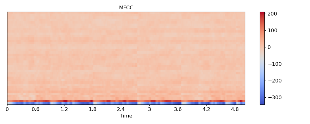
Visualize the MFCC series

>>> import matplotlib.pyplot as plt
>>> plt.figure(figsize=(10, 4))
>>> librosa.display.specshow(mfccs, x_axis='time')
>>> plt.colorbar()
>>> plt.title('MFCC')
>>> plt.tight_layout()
>>> plt.show()

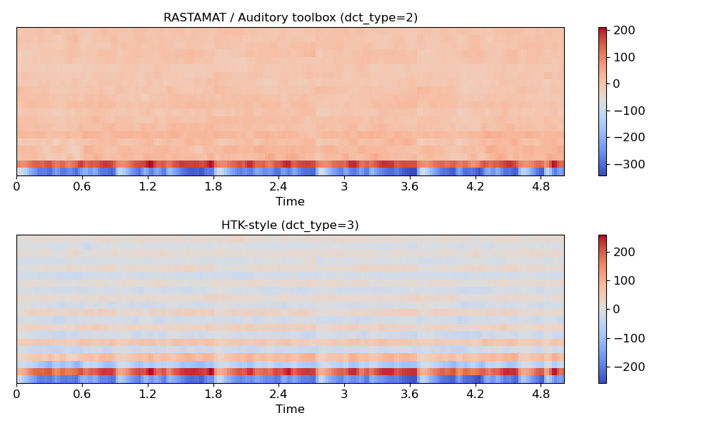
Compare different DCT bases

>>> m_slaney = librosa.feature.mfcc(y=y, sr=sr, dct_type=2)
>>> m_htk = librosa.feature.mfcc(y=y, sr=sr, dct_type=3)
>>> plt.figure(figsize=(10, 6))
>>> plt.subplot(2, 1, 1)
>>> librosa.display.specshow(m_slaney, x_axis='time')
>>> plt.title('RASTAMAT / Auditory toolbox (dct_type=2)')
>>> plt.colorbar()
>>> plt.subplot(2, 1, 2)
>>> librosa.display.specshow(m_htk, x_axis='time')
>>> plt.title('HTK-style (dct_type=3)')
>>> plt.colorbar()
>>> plt.tight_layout()
>>> plt.show()