Caution

You're reading an old version of this documentation. If you want up-to-date information, please have a look at 0.9.1.

librosa.feature.spectral_centroid

librosa.feature.spectral_centroid(y=None, sr=22050, S=None, n_fft=2048, hop_length=512, freq=None, win_length=None, window='hann', center=True, pad_mode='reflect')

Compute the spectral centroid.

Each frame of a magnitude spectrogram is normalized and treated as a distribution over frequency bins, from which the mean (centroid) is extracted per frame.

More precisely, the centroid at frame t is defined as [1]:

centroid[t] = sum_k S[k, t] * freq[k] / (sum_j S[j, t])

where S is a magnitude spectrogram, and freq is the array of frequencies (e.g., FFT frequencies in Hz) of the rows of S.

1

Klapuri, A., & Davy, M. (Eds.). (2007). Signal processing methods for music transcription, chapter 5. Springer Science & Business Media.

Parameters

ynp.ndarray [shape=(n,)] or None

audio time series

srnumber > 0 [scalar]

audio sampling rate of y

Snp.ndarray [shape=(d, t)] or None

(optional) spectrogram magnitude

n_fftint > 0 [scalar]

FFT window size

hop_lengthint > 0 [scalar]

hop length for STFT. See librosa.core.stft for details.

freqNone or np.ndarray [shape=(d,) or shape=(d, t)]

Center frequencies for spectrogram bins. If None, then FFT bin center frequencies are used. Otherwise, it can be a single array of d center frequencies, or a matrix of center frequencies as constructed by librosa.core.ifgram

win_lengthint <= n_fft [scalar]

Each frame of audio is windowed by window(). The window will be of length win_length and then padded with zeros to match n_fft.

If unspecified, defaults to win_length = n_fft.

windowstring, tuple, number, function, or np.ndarray [shape=(n_fft,)]

• a window specification (string, tuple, or number); see scipy.signal.get_window

• a window function, such as scipy.signal.hanning

• a vector or array of length n_fft

centerboolean

• If True, the signal y is padded so that frame t is centered at y[t * hop_length].

• If False, then frame t begins at y[t * hop_length]

pad_modestring

If center=True, the padding mode to use at the edges of the signal. By default, STFT uses reflection padding.

Returns

centroidnp.ndarray [shape=(1, t)]

centroid frequencies

See also

librosa.core.stft

Short-time Fourier Transform

librosa.core.ifgram

Instantaneous-frequency spectrogram

Examples

From time-series input:

>>> y, sr = librosa.load(librosa.util.example_audio_file())
>>> cent = librosa.feature.spectral_centroid(y=y, sr=sr)
>>> cent
array([[ 4382.894,   626.588, ...,  5037.07 ,  5413.398]])

From spectrogram input:

>>> S, phase = librosa.magphase(librosa.stft(y=y))
>>> librosa.feature.spectral_centroid(S=S)
array([[ 4382.894,   626.588, ...,  5037.07 ,  5413.398]])

Using variable bin center frequencies:

>>> y, sr = librosa.load(librosa.util.example_audio_file())
>>> if_gram, D = librosa.ifgram(y)
>>> librosa.feature.spectral_centroid(S=np.abs(D), freq=if_gram)
array([[ 4420.719,   625.769, ...,  5011.86 ,  5221.492]])

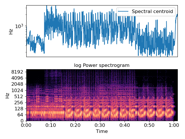
Plot the result

>>> import matplotlib.pyplot as plt
>>> plt.figure()
>>> plt.subplot(2, 1, 1)
>>> plt.semilogy(cent.T, label='Spectral centroid')
>>> plt.ylabel('Hz')
>>> plt.xticks([])
>>> plt.xlim([0, cent.shape[-1]])
>>> plt.legend()
>>> plt.subplot(2, 1, 2)
>>> librosa.display.specshow(librosa.amplitude_to_db(S, ref=np.max),
...                          y_axis='log', x_axis='time')
>>> plt.title('log Power spectrogram')
>>> plt.tight_layout()
>>> plt.show()