librosa.feature.poly_features

librosa.feature.poly_features(*, y=None, sr=22050, S=None, n_fft=2048, hop_length=512, win_length=None, window='hann', center=True, pad_mode='constant', order=1, freq=None)

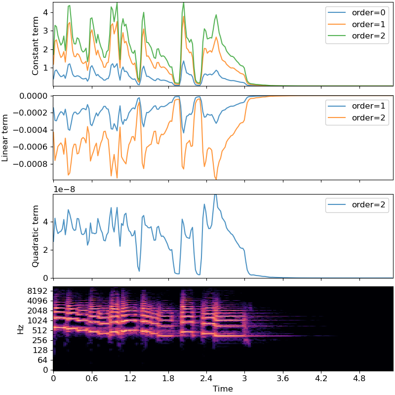
Get coefficients of fitting an nth-order polynomial to the columns of a spectrogram.

Parameters:

ynp.ndarray [shape=(…, n)] or None

audio time series. Multi-channel is supported.

srnumber > 0 [scalar]

audio sampling rate of y

Snp.ndarray [shape=(…, d, t)] or None

(optional) spectrogram magnitude

n_fftint > 0 [scalar]

FFT window size

hop_lengthint > 0 [scalar]

hop length for STFT. See librosa.stft for details.

win_lengthint <= n_fft [scalar]

Each frame of audio is windowed by window(). The window will be of length win_length and then padded with zeros to match n_fft. If unspecified, defaults to win_length = n_fft.

windowstring, tuple, number, function, or np.ndarray [shape=(n_fft,)]

• a window specification (string, tuple, or number); see scipy.signal.get_window

• a window function, such as scipy.signal.windows.hann

• a vector or array of length n_fft

centerboolean

• If True, the signal y is padded so that frame t is centered at y[t * hop_length].

• If False, then frame t begins at y[t * hop_length]

pad_modestring

If center=True, the padding mode to use at the edges of the signal. By default, STFT uses zero padding.

orderint > 0

order of the polynomial to fit

freqNone or np.ndarray [shape=(d,) or shape=(…, d, t)]

Center frequencies for spectrogram bins. If None, then FFT bin center frequencies are used. Otherwise, it can be a single array of d center frequencies, or a matrix of center frequencies as constructed by librosa.reassigned_spectrogram

Returns:

coefficientsnp.ndarray [shape=(…, order+1, t)]

polynomial coefficients for each frame.

coefficients[..., 0, :] corresponds to the highest degree (order),

coefficients[..., 1, :] corresponds to the next highest degree (order-1),

down to the constant term coefficients[..., order, :].

Examples

>>> y, sr = librosa.load(librosa.ex('trumpet'))
>>> S = np.abs(librosa.stft(y))

Fit a degree-0 polynomial (constant) to each frame

>>> p0 = librosa.feature.poly_features(S=S, order=0)

Fit a linear polynomial to each frame

>>> p1 = librosa.feature.poly_features(S=S, order=1)

Fit a quadratic to each frame

>>> p2 = librosa.feature.poly_features(S=S, order=2)

Plot the results for comparison

>>> import matplotlib.pyplot as plt
>>> fig, ax = plt.subplots(nrows=4, sharex=True, figsize=(8, 8))
>>> times = librosa.times_like(p0)
>>> ax[0].plot(times, p0[0], label='order=0', alpha=0.8)
>>> ax[0].plot(times, p1[1], label='order=1', alpha=0.8)
>>> ax[0].plot(times, p2[2], label='order=2', alpha=0.8)
>>> ax[0].legend()
>>> ax[0].label_outer()
>>> ax[0].set(ylabel='Constant term ')
>>> ax[1].plot(times, p1[0], label='order=1', alpha=0.8)
>>> ax[1].plot(times, p2[1], label='order=2', alpha=0.8)
>>> ax[1].set(ylabel='Linear term')
>>> ax[1].label_outer()
>>> ax[1].legend()
>>> ax[2].plot(times, p2[0], label='order=2', alpha=0.8)
>>> ax[2].set(ylabel='Quadratic term')
>>> ax[2].legend()
>>> librosa.display.specshow(librosa.amplitude_to_db(S, ref=np.max),
...                          y_axis='log', x_axis='time', ax=ax[3])