librosa.feature.spectral_contrast

librosa.feature.spectral_contrast(*, y=None, sr=22050, S=None, n_fft=2048, hop_length=512, win_length=None, window='hann', center=True, pad_mode='constant', freq=None, fmin=200.0, n_bands=6, quantile=0.02, linear=False)

Compute spectral contrast

Each frame of a spectrogram S is divided into sub-bands. For each sub-band, the energy contrast is estimated by comparing the mean energy in the top quantile (peak energy) to that of the bottom quantile (valley energy). High contrast values generally correspond to clear, narrow-band signals, while low contrast values correspond to broad-band noise. [1]

[1]

Jiang, Dan-Ning, Lie Lu, Hong-Jiang Zhang, Jian-Hua Tao, and Lian-Hong Cai. “Music type classification by spectral contrast feature.” In Multimedia and Expo, 2002. ICME’02. Proceedings. 2002 IEEE International Conference on, vol. 1, pp. 113-116. IEEE, 2002.

Parameters:

ynp.ndarray [shape=(…, n)] or None

audio time series. Multi-channel is supported.

srnumber > 0 [scalar]

audio sampling rate of y

Snp.ndarray [shape=(…, d, t)] or None

(optional) spectrogram magnitude

n_fftint > 0 [scalar]

FFT window size

hop_lengthint > 0 [scalar]

hop length for STFT. See librosa.stft for details.

win_lengthint <= n_fft [scalar]

Each frame of audio is windowed by window(). The window will be of length win_length and then padded with zeros to match n_fft. If unspecified, defaults to win_length = n_fft.

windowstring, tuple, number, function, or np.ndarray [shape=(n_fft,)]

• a window specification (string, tuple, or number); see scipy.signal.get_window

• a window function, such as scipy.signal.windows.hann

• a vector or array of length n_fft

centerboolean

• If True, the signal y is padded so that frame t is centered at y[t * hop_length].

• If False, then frame t begins at y[t * hop_length]

pad_modestring

If center=True, the padding mode to use at the edges of the signal. By default, STFT uses zero padding.

freqNone or np.ndarray [shape=(d,)]

Center frequencies for spectrogram bins. If None, then FFT bin center frequencies are used. Otherwise, it can be a single array of d center frequencies.

fminfloat > 0

Frequency cutoff for the first bin [0, fmin] Subsequent bins will cover [fmin, 2*fmin]`, `[2*fmin, 4*fmin], etc.

n_bandsint > 1

number of frequency bands

quantilefloat in (0, 1)

quantile for determining peaks and valleys

linearbool

If True, return the linear difference of magnitudes: peaks - valleys. If False, return the logarithmic difference: log(peaks) - log(valleys).

Returns:

contrastnp.ndarray [shape=(…, n_bands + 1, t)]

each row of spectral contrast values corresponds to a given octave-based frequency

Examples

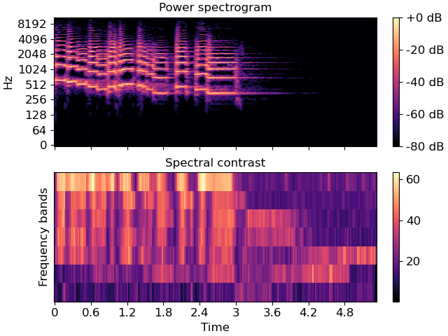
>>> y, sr = librosa.load(librosa.ex('trumpet'))
>>> S = np.abs(librosa.stft(y))
>>> contrast = librosa.feature.spectral_contrast(S=S, sr=sr)

>>> import matplotlib.pyplot as plt
>>> fig, ax = plt.subplots(nrows=2, sharex=True)
>>> img1 = librosa.display.specshow(librosa.amplitude_to_db(S,
...                                                  ref=np.max),
...                          y_axis='log', x_axis='time', ax=ax[0])
>>> fig.colorbar(img1, ax=[ax[0]], format='%+2.0f dB')
>>> ax[0].set(title='Power spectrogram')
>>> ax[0].label_outer()
>>> img2 = librosa.display.specshow(contrast, x_axis='time', ax=ax[1])
>>> fig.colorbar(img2, ax=[ax[1]])
>>> ax[1].set(ylabel='Frequency bands', title='Spectral contrast')