Caution

You're reading the documentation for a development version. For the latest released version, please have a look at 0.11.0.

librosa.display.wavebars

librosa.display.wavebars(y, *, sr=22050, n_bars=100, gap_ratio=0.4, rounding_ratio=0.5, axis='time', offset=0.0, invert=False, invert_color=None, transpose=False, label=None, ax=None, **patch_kwargs)

Visualize a waveform as a series of bars representing the amplitude envelope.

This visualization is appropriate for displaying a simplified view of the signal, and is best suited for small figures where simplicity is desired.

Parameters:

ynp.ndarray [shape=(n,) or (2,n)]

audio time series (mono or stereo) If stereo, the left channel’s amplitude envelope will be used for the top of the bars, and the right channel’s amplitude envelope (negated) will be used for the bottom of the bars. If mono, the signal’s envelope is mirrored across the axis.

srnumber > 0 [scalar]

sampling rate of y (samples per second)

n_barsint > 0

Number of bars to display in the waveform plot. The total time extent of the plot will be divided into n_bars segments, and the amplitude envelope of each segment will be represented as a bar.

gap_ratiofloat in [0, 1]

The fraction of the bar width that will be left as a gap between adjacent bars.

rounding_ratiofloat in [0, 1]

The fraction of the bar width that will be used for rounding the corners of the bars. A value of 0.5 will produce bars with rounded corners, while a value of 0 will produce rectangular bars.

axisstr or None

Display style of the axis ticks and tick markers. Accepted values are:

• ‘time’ : markers are shown as milliseconds, seconds, minutes, or hours.

• ‘h’ : markers are shown as hours, minutes, and seconds.

• ‘m’ : markers are shown as minutes and seconds.

• ‘s’ : markers are shown as seconds.

• ‘ms’ : markers are shown as milliseconds.

• ‘lag’ : like time, but past the halfway point counts as negative values.

• ‘lag_h’ : same as lag, but in hours.

• ‘lag_m’ : same as lag, but in minutes.

• ‘lag_s’ : same as lag, but in seconds.

• ‘lag_ms’ : same as lag, but in milliseconds.

• None, ‘none’, or ‘off’: ticks and tick markers are hidden.

offsetfloat

Offset (in seconds) to start the waveform plot.

invertbool

If True, invert the foreground and background of the display, so that the axes background is colored. If False (default), the envelope display is colored and the background is unchanged.

invert_colorstr, tuple, None

If invert is True, this parameter specifies the color to use for the inverted waveform display. If None (default), the color is set to the current axes background color.

transposebool

If True, display the wave vertically instead of horizontally.

labelstr or None

The label string applied to this plot. If None, no label is applied.

axmatplotlib.axes.Axes or None

Axes to plot on instead of the default plt.gca().

**patch_kwargsdict

Additional keyword arguments to pass to matplotlib.patches.FancyBboxPatch

Returns:

matplotlib.collections.PatchCollection

A collection of patches representing the amplitude envelope of the waveform.

See also

waveshow

Examples

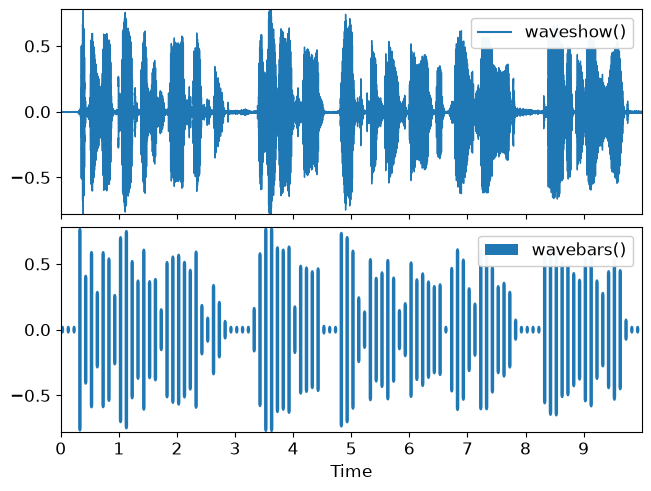
Plot a waveform as bars, compared to the waveshow version of the plot

>>> import matplotlib.pyplot as plt
>>> y, sr = librosa.loadx('libri1', duration=10)
>>> fig, ax = plt.subplots(nrows=2, sharex=True)
>>> librosa.display.waveshow(y=y, sr=sr, ax=ax[0], label='waveshow()')
>>> ax[0].legend()
>>> ax[0].label_outer()
>>> librosa.display.wavebars(y=y, sr=sr, ax=ax[1], label='wavebars()')
>>> ax[1].legend()
>>> plt.show()

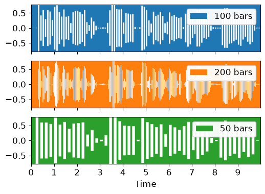
Make plots with varying amounts of detail, squared corners, and inverted colors.

>>> fig, ax = plt.subplots(nrows=3, sharex=True, sharey=True)
>>> librosa.display.wavebars(y=y, sr=sr, n_bars=100, rounding_ratio=0,
...                          invert=True, ax=ax[0], label='100 bars')
>>> librosa.display.wavebars(y=y, sr=sr, n_bars=200, rounding_ratio=0,
...                          color='C1', invert=True, ax=ax[1], label='200 bars')
>>> librosa.display.wavebars(y=y, sr=sr, n_bars=50, rounding_ratio=0,
...                          color='C2', invert=True, ax=ax[2], label='50 bars')
>>> ax[0].legend()
>>> ax[1].legend()
>>> ax[2].legend()
>>> ax[0].label_outer()
>>> ax[1].label_outer()
>>> plt.show()