Caution

You're reading the documentation for a development version. For the latest released version, please have a look at 0.11.0.

librosa.display.wavef0

librosa.display.wavef0(y, *, f0, sr=22050, hop_length=512, bins_per_octave=12, time_axis='time', freq_axis='cqt_note', offset=0.0, key='C:maj', Sa=None, mela=None, thaat=None, unicode=True, ax=None, method='waveshow', transpose=False, **kwargs)

Visualize a waveform with an f0-displacement.

This can be used to simultaneously visualize the fundamental frequency (f0) estimates and the waveform or amplitude envelope of an audio signal in one compact display.

Parameters:

ynp.ndarray [shape=(n,) or (2,n)]

audio time series (mono or stereo) If stereo, the left channel’s amplitude envelope will be used for the top of the plot, and the right channel’s amplitude envelope (negated) will be used for the bottom of the plot. If mono, the signal’s envelope is mirrored across the axis.

f0np.ndarray [shape=(m,)]

Fundamental frequency (f0) estimates in Hz. This should be computed using a pitch estimation algorithm such as librosa.pyin or librosa.yin.

srnumber > 0 [scalar]

sampling rate of y (samples per second)

hop_lengthint > 0

Hop length (in samples) between successive f0 estimates. This should match the hop length used to compute f0.

bins_per_octaveint > 0

Number of frequency bins per octave used to scale the waveform’s amplitude displacement around f0. Combined with the waveform’s peak amplitude (used as the displacement norm), this controls how many bins of vertical displacement correspond to one octave above or below f0.

time_axisstr

Display style of the time axis ticks and tick markers. Accepted values are:

• ‘time’ : markers are shown as milliseconds, seconds, minutes, or hours.

• ‘h’ : markers are shown as hours, minutes, and seconds.

• ‘m’ : markers are shown as minutes and seconds.

• ‘s’ : markers are shown as seconds.

• ‘ms’ : markers are shown as milliseconds.

• ‘lag’ : like time, but past the halfway point counts as negative values.

• ‘lag_h’ : same as lag, but in hours.

• ‘lag_m’ : same as lag, but in minutes.

• ‘lag_s’ : same as lag, but in seconds.

• ‘lag_ms’ : same as lag, but in milliseconds.

• None, ‘none’, or ‘off’: ticks and tick markers are hidden.

freq_axisstr

Display style of the frequency axis ticks and tick markers. Accepted values are:

• ‘cqt_note’ : markers are shown as note names.

• ‘cqt_hz’ : markers are shown as frequencies in Hz.

• ‘cqt_oct3’ : markers are shown in Hz using 1/3-octave intervals.

• ‘cqt_svara’ : markers are shown as Indian classical music svara names.

offsetfloat

Offset (in seconds) to start the waveform plot.

keystr

Key signature for the frequency axis. This is used to determine the note names for the frequency axis when using cqt_note mode.

Safloat or None

Sa (tonic) frequency in Hz for the frequency axis. Required for cqt_svara mode.

melastr or int or None

Mela (scale) name or index for the frequency axis. This is used to determine the svara names for the frequency axis when using cqt_svara mode.

thaatstr or None

Thaat (scale) name for the frequency axis. This is used to determine the svara names for the frequency axis when using cqt_svara mode.

unicodebool

If True, use Unicode characters for frequency axis labels.

axmatplotlib.axes.Axes or None

Axes to plot on instead of the default plt.gca().

methodstr

Method to use for visualizing the waveform with f0 displacement. Accepted values are:

• ‘waveshow’ : Use librosa.display.waveshow to visualize the waveform with an f0 displacement.

• ‘wavebars’ : Use librosa.display.wavebars to visualize the waveform as bars with an f0 displacement.

transposebool

If True, display the wave vertically instead of horizontally.

**kwargsdict

Additional keyword arguments forwarded to the plotting function selected by method.

If method=’waveshow’, these must be keyword arguments supported by librosa.display.waveshow (for example, max_points).

If method=’wavebars’, these must be keyword arguments supported by librosa.display.wavebars (for example, n_bars, gap_ratio, rounding_ratio, invert, and invert_color).

Keyword arguments for one method are not valid when using the other.

Returns:

AdaptiveWaveplot or PatchCollection

An object of type librosa.display.AdaptiveWaveplot if method=’waveshow’, or a matplotlib.collections.PatchCollection if method=’wavebars’.

See also

waveshow

wavebars

Examples

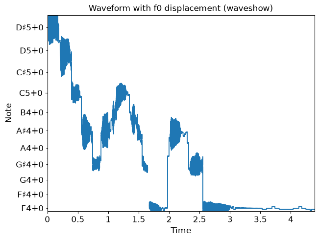
Visualize a waveform with an f0 displacement using waveshow

>>> import matplotlib.pyplot as plt
>>> y, sr = librosa.loadx('trumpet')
>>> f0, _, _ = librosa.pyin(y, fmin=librosa.note_to_hz('C2'),
...                         fmax=librosa.note_to_hz('C7'),
...                         sr=sr, hop_length=512)
>>> fig, ax = plt.subplots()
>>> librosa.display.wavef0(y=y, f0=f0, sr=sr, ax=ax,
...                        method='waveshow')
>>> ax.set(title='Waveform with f0 displacement (waveshow)')
>>> plt.show()

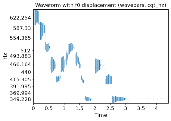
Visualize a waveform with an f0 displacement using wavebars, and Hz labels instead of note names. Using a larger number of bars shows more detail here.

>>> fig, ax = plt.subplots()
>>> librosa.display.wavef0(y=y, f0=f0, sr=sr, ax=ax, n_bars=256,
...                        method='wavebars', freq_axis='cqt_hz')
>>> ax.set(title='Waveform with f0 displacement (wavebars, cqt_hz)')
>>> plt.show()

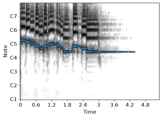
Overlay a displaced waveform on a CQT plot via specshow.

>>> fig, ax = plt.subplots()
>>> C = librosa.cqt(y, sr=sr)
>>> librosa.display.specshow(C, ax=ax, sr=sr, x_axis='time', y_axis='cqt_note',
...                          vscale='dBFS', cmap='gray_r')
>>> hl = librosa.display.highlight(ax=ax)
>>> librosa.display.wavef0(y=y, f0=f0, sr=sr, ax=ax, path_effects=hl)