Getting started with audio data

This section introduces the basics of loading audio with librosa.

Loading an audio file

To get started, we can use some of the example recordings that come bundled with librosa. These are available through the librosa.example function, which fetches the data from the web and caches it locally.

Before we do anything else, we’ll need to import the library:

import librosa
from IPython.display import HTML  # this is for displaying metadata about the example

Next, we’ll load an example audio file. We’ll use the “trumpet” example to start with, but there are many others available. You can see a list of available examples by calling librosa.util.list_examples().

filename = librosa.example("trumpet")

y, sr = librosa.load(filename)

# And print out some information about this example
HTML(librosa.util.example_info("trumpet", html=True))

solo trumpet 06

By: Mihai Sorohan | License: CC-BY-4.0

Source: https://freesound.org/s/77711/

Description

Part of "Jazz Trumpet Loops Pack in F 90 bpm" by Mihai Sorohan
All parts in this pack are in F, mostly Blues and Dorian scale and all are in stereo acidized .wav format, 16 bit, 44.1 khz sample rate, 90 bpm.

Gear used:
- trumpet Bb Amati ATR213
- microphone Oktava MK 319
- preamp Art Tube MP Project Series
- soundcard M-Audio Delta Audiophile 192

Caution

In this section, we use librosa.load directly. Elsewhere in the documentation, you may see librosa.loadx, which is a convenience wrapper for loading bundled example audio.

For your own files, use librosa.load.

We now have our audio signal loaded as an array of samples stored in y, and the sampling rate (samples per second) stored in sr. If you print these out, you should see something like the following:

print("y:", y)

y: [-0.001 -0.    -0.    ...  0.    -0.     0.   ]

print("sr:", sr)

sr: 22050

Working with digital audio samples

By default, librosa.load will standardize the signal to a sampling rate of 22050 samples per second, and downmix stereo signals to mono. You can customize this behavior by specifying the sr and mono arguments, respectively. To use the audio file’s native sampling rate, simply set sr=None.

For now, we’ll stick with the default settings of mono and sr=22050. These are designed to work well with the rest of the default parameters in librosa, and should be suitable for most analysis tasks. This has the added benefit that any subsequent processing steps will behave consistently for different example inputs, which may be recorded at different sampling rates.

The variable y is an audio time series, encoded as a one-dimensional NumPy array. Each element in the array is a floating point number representing the value of the audio signal at the corresponding sample position. These values correspond to the fluctuations in air pressure that we perceive as sound.

The sampling rate sr tells us how many samples we have every second, in this case, 22050. To see how many samples we have in total, we can print the shape of the audio array:

print("number of samples: ", y.shape)

number of samples:  (117601,)

To find the duration of the audio signal in seconds, we can divide the number of samples by the sampling rate:

print("duration (s): ", y.shape[0] / sr)

duration (s):  5.333378684807256

Librosa also provides a helper function that can compute the duration of a signal for us, given the signal itself and the sampling rate:

print("duration (s): ", librosa.get_duration(y=y, sr=sr))

duration (s):  5.333378684807256

Similarly, if we want to find the time value corresponding to a given sample index, we can use the librosa.samples_to_time function:

print("time (s) at sample 100: ", librosa.samples_to_time(100, sr=sr))

time (s) at sample 100:  0.0045351473922902496

Plotting the signal

We can visualize the audio signal by plotting the samples. Librosa provides several utilities for visualizing audio data, and builds upon the matplotlib package. While it is possible to use matplotlib directly to plot the signal, librosa has a built-in function librosa.display.waveshow that simplifies the process and avoids some common difficulties.

We’ll need to import matplotlib first:

import matplotlib.pyplot as plt

We can then use standard matplotlib commands to create a figure, and librosa.display to draw the waveform on it.

# Construct a figure and axes object:
fig, ax = plt.subplots()

# Plot on the axes:
librosa.display.waveshow(y, sr=sr, ax=ax)

# Set the title for the figure
ax.set(title="Trumpet example")

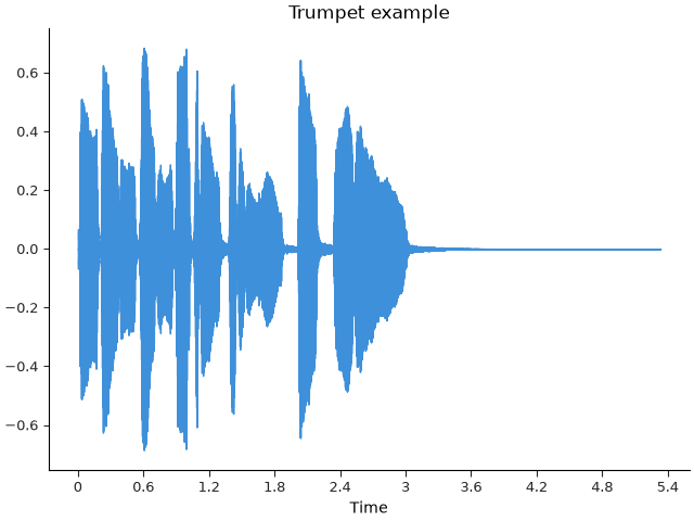
The waveshow function provides some useful defaults for plotting audio signals, and sets the horizontal axis to be time (measured in seconds).

Listening to the audio

Finally, we can listen to the audio signal that we’ve loaded. To do this, we’ll use the IPython.display.Audio class. Note that this will only work if you’re running this code in a browser-based environment, such as Jupyter notebook.

To play audio in the browser, we’ll need to import the Audio class from the IPython.display module:

from IPython.display import Audio

We can then use the Audio class to create an audio player, and the display function to render it:

Audio(data=y, rate=sr)

Note: when using browser-based playback in a notebook environment, the Audio(…) command must be the last line in the cell. Otherwise, the notebook will not display the player widget. To force the player to display, you can use the display function from IPython.display, like shown below. This can be used to show multiple players in the same cell.

from IPython.display import display
display(Audio(data=y, rate=sr))

<IPython.lib.display.Audio object>

Summary

In this notebook, we’ve seen how to do the following: 1. Load an audio file using librosa.load 2. Understand the sampling rate and duration of the audio signal 3. Visualize the audio signal using matplotlib and librosa.display.waveshow 4. Listen to the audio signal using IPython.display.Audio

In the next section, we’ll see how to extract useful information from the audio signal.