Non-uniform coordinate grids

This section demonstrates how to explicitly set coordinate positions to visualize data with non-uniform spacing, such as beat-synchronous features in music.

Usually when visualizing audio data, the axes of visualizations have predictable spacing. For example, waveforms usually have uniform time spacing between samples (as determined by the sampling rate), and spectrograms have either uniform spacing of frequency bins (if using a Fourier analysis), geometric spacing (if using a Constant-Q analysis), etc.

Sometimes, you may want to visualize data that has non-uniform spacing, but still retain the proper coordinate positions in the display. librosa.display.specshow supports this by allowing you to explicitly set the coordinates of the axes using the x_coords and y_coords parameters.

A simple use-case of this is to visualize beat-synchronous features, where the time axis is defined by the beat positions rather than the sample indices. Let’s first compute uniformly spaced and beat-synchronous features to illustrate how this looks.

import librosa
import numpy as np
import matplotlib.pyplot as plt
from IPython.display import HTML

y, sr = librosa.loadx("brahms")
HTML(librosa.util.example_info("brahms", html=True))

Hungarian Dance number 5

By: Johannes Brahms (composer), US Army Strings (performer) | License: CC-PDM-1.0

Source: https://musopen.org/music/43805-hungarian-dance-no-5-in-f-sharp-minor-woo-1-string-orch

Description

An excerpt of Hungarian Dance number 5 in F♯ minor by Johannes Brahms,
arranged for string orchestra and performed by the US Army Strings.

chroma = librosa.feature.chroma_cqt(y=y, sr=sr, threshold=2)
tempo, beats = librosa.beat.beat_track(y=y, sr=sr, trim=False)

Now beats contains the frame indices of detected beats. To ensure that we have full coverage of the audio, we can add the beginning (frame 0) to the beat array and use librosa.util.sync to aggregate chroma features over each interval.

beats = librosa.util.fix_frames(beats, x_min=0)
chroma_sync = librosa.util.sync(chroma, beats, aggregate=np.median)

fig, ax = plt.subplots(nrows=2)
librosa.display.specshow(chroma, y_axis="chroma", x_axis="time", ax=ax[0])
ax[0].set(title="Uniformly sampled chroma", xlabel=None)
librosa.display.specshow(chroma_sync, y_axis="chroma", ax=ax[1])
ax[1].set(title="Beat-synchronous chroma", xlabel=None)

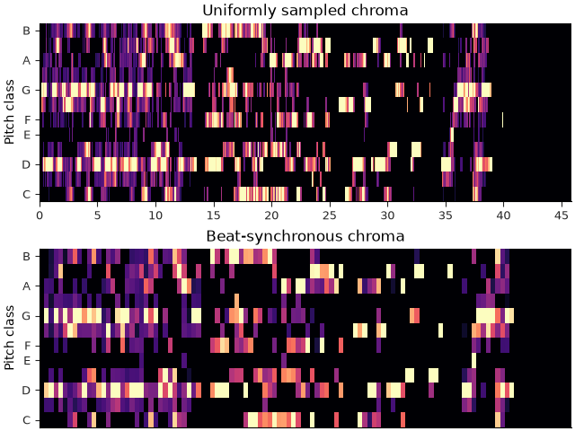
The figure above basically works, but the horizontal axes are using completely distinct layouts: the top uses units of seconds, while the bottom uses units of beat indices (0, 1, 2, …). More importantly, the non-uniformity of beat spacing results in significant drift between the visual representations of the two subplots, which is especially evident in the final region of the upper plot beginning at around 35 seconds.

We can fix this by explicitly setting the x_coords parameter of the second specshow call to the beat times, which we can compute using librosa.frames_to_time. When providing x_coords, the length of the coordinate array should match that of the data being displayed:

# Convert beat frames to times
beat_times = librosa.frames_to_time(beats, sr=sr)
print(f"chroma_sync.shape = {chroma_sync.shape}\nbeat_times.shape = {beat_times.shape}")

chroma_sync.shape = (12, 112)
beat_times.shape = (112,)

fig, ax = plt.subplots(nrows=2, sharex=True, sharey=True)
librosa.display.specshow(chroma, y_axis="chroma", x_axis="time", ax=ax[0])
ax[0].set(title="Uniformly sampled chroma", xlabel=None)

librosa.display.specshow(chroma_sync, y_axis="chroma",
                         x_coords=beat_times, x_axis="time",
                         ax=ax[1])
ax[1].set(title="Beat-synchronous chroma", xlabel=None)

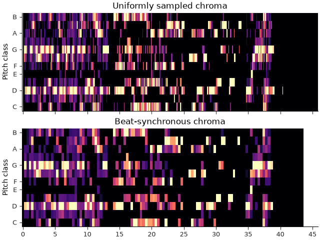
Now the two subplots are aligned in time, and we can also use the x_axis=’time’ parameter to automatically format the x-axis ticks in seconds using the provided coordinates instead of assuming uniform sampling. Note that the beat-synchronous plot appears to stop early: this is because the data is only defined up to the final beat position.

Summary

Explicit coordinate positions can be used in any specshow display, and the functionality is not limited to time-like axes. Rather, every x_axis= or y_axis= setting involves some calculation of the corresponding coordinate grid, and the x_coords and y_coords parameters allow you to override those calculations with your own coordinate positions for highly customized displays. Generally, you will still want to use the x_axis= and y_axis= parameters to automatically format the axes for you.