Rhythm analysis

This section covers methods for estimating tempo and beat positions from audio signals.

The previous section introduced methods for identifying the positions of note onsets. In this section, we build on onset detection to answer two rhythm-related questions: how fast is the pulse, and where do the beats occur?

import librosa
import numpy as np
import matplotlib.pyplot as plt
import matplotlib.animation as animation
from IPython.display import Audio, HTML

# Load an example audio file with a beat
y, sr = librosa.loadx("sweetwaltz", duration=20.0)
HTML(librosa.util.example_info("sweetwaltz", html=True))

Sweet Waltz

By: setuniman | License: CC-BY-NC-4.0

Source: https://freesound.org/people/Setuniman/sounds/147793/

Description

Steady change between two naive major phrases beginning with wooden timbre is gradually layered by flute and organ colours. Made with synths.

Audio(url=librosa.util.example("sweetwaltz", url=True))

The starting point for rhythm analysis is often the onset strength envelope. We often use the envelope rather than detected onset positions to avoid error propagation from incorrect detections.

First, let’s visualize the audio signal, its spectrogram, and the onset strength envelope.

onset_env = librosa.onset.onset_strength(y=y, sr=sr)
times = librosa.times_like(onset_env, sr=sr)
S = librosa.stft(y)

fig, ax = plt.subplots(nrows=3, sharex=True, height_ratios=(1, 1, 2))
ax[0].plot(times, onset_env, label="Onset strength", color="C1")
librosa.display.waveshow(y, sr=sr, ax=ax[1], label="Waveform")
img = librosa.display.specshow(S, sr=sr, vscale="dBFS", x_axis="time", y_axis="log", ax=ax[2])
librosa.display.colorbar_db(img, label="dBFS")
ax[0].legend(loc="upper right")
ax[1].legend(loc="upper right")
ax[0].label_outer()
ax[1].label_outer()

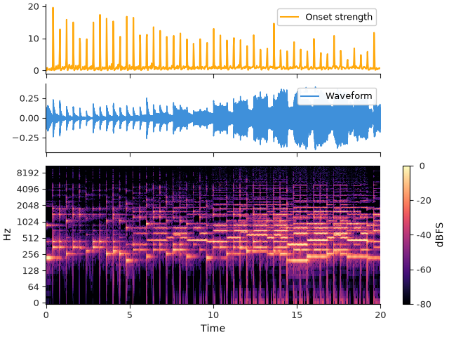
The onset strength envelope displayed above contains many peaks, which correspond to musical onsets. In this example, the peaks are also regularly spaced in time. When we listen to this example this regular spacing is perceived as a pulse or beat. After computing the onset strength, the next step in rhythm analysis is often to estimate the tempo, that is, the time spacing of the pulse.

Estimating the tempo

A typical method for estimating tempo from the onset strength envelope is to compute the autocorrelation of the envelope, which measures how similar the envelope is to a delayed copy of itself. The animation below illustrates this process, limited to the first 5 seconds of the audio signal.

fig, ax = plt.subplots(nrows=2)
times = librosa.times_like(onset_env, sr=sr)
ax[0].plot(times, onset_env, label="Onset strength", color="C1")
onset_delayed = ax[0].plot(times, onset_env, label="Delayed onset strength", color="C4", linestyle="--")[0]

ax[0].set(xlim=(0, 5), xlabel="Time (s)")
ax[0].legend(loc="upper right")

xcorr = np.correlate(onset_env, onset_env, mode="same")
corrplot = ax[1].plot(times, xcorr, label="Autocorrelation", color="C2")[0]
ax[1].legend(loc="upper right")
ax[1].set(xlim=(0, 5), xlabel="Lag (s)")

def _update(num):
    """Update the plot for each frame."""
    # Update the delayed onset strength
    # Show the onset strength envelope delayed by `num` frames
    onset_delayed.set_xdata(times + num * times[1])
    # Show the autocorrelation up to the current amount of lag
    corrplot.set_xdata(times[:num])
    corrplot.set_ydata(xcorr[:num])
    return (onset_delayed, corrplot)

ani = animation.FuncAnimation(fig,
                              func=_update,
                              frames=int(np.ceil(5 / times[1]).astype(int)),
                              interval=50,
                              blit=True)

Once Loop Reflect

The tempo is determined by the position of the first prominent peak in the autocorrelation, not including the peak at lag of zero. In this example, the first peak occurs at around 0.4 seconds. Interpreted as a repeating period, this lag corresponds to a pulse rate of 2.5 cycles per second, or 150 beats per minute. More often, tempo is expressed in units of beats per minute (BPM), rather than cycles per second (Hz), and we can convert between the two by multiplying by 60. This calculation results in a tempo of 150 BPM.

Of course, librosa provides a convenient function to compute the tempo directly, either from the signal y or from a pre-computed onset strength envelope.

tempo = librosa.feature.tempo(onset_envelope=onset_env, sr=sr)
print(f"Estimated tempo: {tempo[0]:.2f} BPM")

Estimated tempo: 152.00 BPM

Behind the scenes, the tempo estimator will compute auto-correlation on short fragments of the onset envelope, and estimate an independent tempo from each fragment. If we collect these autocorrelation results together, we can visualize the data as a tempogram, just like we did previously for spectrograms, and plot the estimated tempo over top.

tgram = librosa.feature.tempogram(onset_envelope=onset_env, sr=sr)
fig, ax = plt.subplots()
librosa.display.specshow(tgram, x_axis="time", y_axis="tempo", sr=sr, ax=ax, cmap_seq="magma")
hl = librosa.display.highlight(ax=ax, alpha=0.95, linewidth=8)
ax.axhline([tempo], label="Estimated tempo",
           path_effects=hl, linewidth=4, linestyle="--")
ax.legend(loc="upper right")

From tempo to beats

So far, we’ve seen how to estimate tempo from the onset strength envelope. This tells us roughly the speed at which beats (typically quarter-notes, ♩) occur, but it does not identify where they occur: that is the job of a beat tracker.

Librosa’s main beat tracker is based on the method of Ellis [1].

[1]

Daniel P. W. Ellis, “Beat Tracking by Dynamic Programming,” Journal of New Music Research, vol. 36, no. 1, pp. 51-60, March 2007.

It essentially works as follows:

1. Estimate the tempo of the recording. This can be either static or dynamic, as described above. 2. Identify peaks in the onset envelope which are approximately spaced by the tempo. 3. Globally optimize the selection of onset envelope peaks subject to tempo constraints.

If a tempo is not provided to the tracker, it will be estimated from the signal directly. Either way, the tracker returns both the tempo estimate and the identified beat positions. Like the onset detector, we can select the units applied to the beat tracker’s estimates: frame indices (default), sample indices, or time (seconds).

tempo, beats = librosa.beat.beat_track(onset_envelope=onset_env, sr=sr, units="time")
print(f"Estimated tempo: {tempo}")
print(f"Estimated beats: {beats}")

Estimated tempo: [151.999]
Estimated beats: [ 0.418  0.836  1.231  1.625  2.02   2.438  2.833  3.228  3.622  4.017
  4.435  4.83   5.224  5.619  6.037  6.432  6.827  7.221  7.639  8.034
  8.429  8.824  9.218  9.636 10.031 10.426 10.82  11.238 11.633 12.028
 12.423 12.817 13.235 13.63  14.025 14.42  14.838 15.232 15.627 16.022
 16.44  16.834 17.229 17.624 18.042 18.437 18.831 19.226 19.621]

We can play back the estimated beats with a click track:

beats_click = librosa.clicks(times=beats, sr=sr, length=len(y))
Audio(data=librosa.to_stereo(left=y, right=beats_click), rate=sr)

And we can also visualize the results by plotting over the onset envelope. This can be done directly with matplotlib, or using the display helpers included in the mir_eval package. For this example, we’ll use mir_eval, and zoom in on the middle ten seconds of the recording.

import mir_eval.display

fig, ax = plt.subplots()
ax.plot(times, onset_env, label="Onset envelope", color="C1")
mir_eval.display.events(beats, ax=ax, label="Beats", linestyle="--")
ax.legend(loc="upper right")
ax.set(xlim=[5, 15])