Enhanced chroma and chroma variants

This notebook demonstrates a variety of techniques for enhancing chroma features and also, introduces chroma variants implemented in librosa.

Enhanced chroma

Beyond the default parameter settings of librosa’s chroma functions, we apply the following enhancements:

1. Harmonic-percussive-residual source separation to eliminate transients.

2. Nearest-neighbor smoothing to eliminate passing tones and sparse noise. This is inspired by the recurrence-based smoothing technique of Cho and Bello, 2011 [1].

3. Local median filtering to suppress remaining discontinuities.

[1]

Taemin Cho & Juan Pablo Bello. (2011). A Feature Smoothing Method for Chord Recognition Using Recurrence Plots. Proceedings of the 12th International Society for Music Information Retrieval Conference, 651–656. https://doi.org/10.5281/zenodo.1417557

Code source: Brian McFee License: ISC sphinx_gallery_thumbnail_number = 5

import numpy as np
import scipy
import matplotlib.pyplot as plt
from IPython.display import Audio, HTML

import librosa

We’ll use a track that has harmonic, melodic, and percussive elements

y, sr = librosa.loadx("fishin")
HTML(librosa.util.example_info("fishin", html=True))

Let's Go Fishin'

By: Karissa Hobbs | License: CC-BY-NC-SA-4.0

Source: https://freemusicarchive.org/music/Karissa_Hobbs/Age_of_Flowers/09_Lets_Go_Fishin/

Description

A pop / folk song with vocals.

Audio(url=librosa.example("fishin", url=True))

First, let’s plot the original chroma

chroma_orig = librosa.feature.chroma_cqt(y=y, sr=sr)

# For display purposes, let's zoom in on a 15-second chunk from the middle of the song
idx = tuple([slice(None), slice(*list(librosa.time_to_frames([45, 60])))])

# And for comparison, we'll show the CQT matrix as well.
C = np.abs(librosa.cqt(y=y, sr=sr, bins_per_octave=12*3, n_bins=7*12*3))


fig, ax = plt.subplots(nrows=2, sharex=True)
img1 = librosa.display.specshow(C[idx], vscale="dBFS",
                                y_axis="cqt_note", x_axis="time", bins_per_octave=12*3,
                                ax=ax[0])
librosa.display.colorbar_db(img1, ax=ax[0])
ax[0].label_outer()

img2 = librosa.display.specshow(chroma_orig[idx], y_axis="chroma", x_axis="time", ax=ax[1])
fig.colorbar(img2, ax=[ax[1]])
ax[1].set(ylabel="Default chroma")

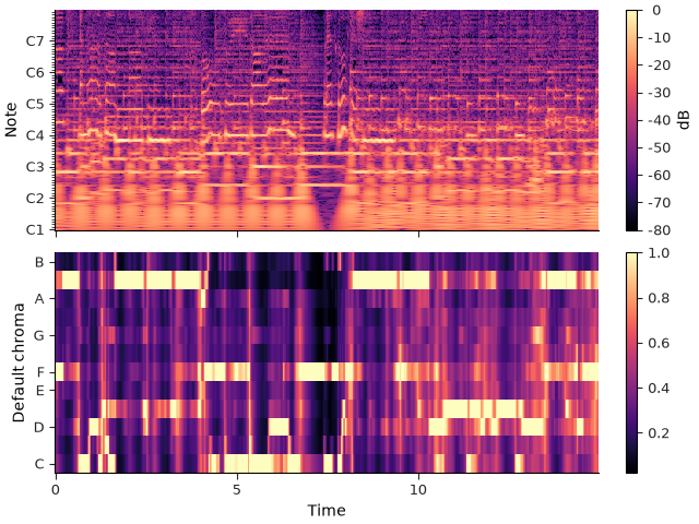
We can do better by isolating the harmonic component of the audio signal. We’ll use a large margin for separating harmonics from percussives:

y_harm = librosa.effects.harmonic(y=y, margin=8)
chroma_harm = librosa.feature.chroma_cqt(y=y_harm, sr=sr)


fig, ax = plt.subplots(nrows=2, sharex=True, sharey=True)
librosa.display.specshow(chroma_orig[idx], y_axis="chroma", x_axis="time", ax=ax[0])
ax[0].set(ylabel="Default chroma")
ax[0].label_outer()

librosa.display.specshow(chroma_harm[idx], y_axis="chroma", x_axis="time", ax=ax[1])
ax[1].set(ylabel="Harmonic")

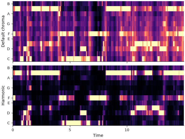
There’s still some noise in there though. We can clean it up using non-local filtering. This effectively removes any sparse additive noise from the features.

chroma_filter = np.minimum(chroma_harm,
                           librosa.decompose.nn_filter(chroma_harm,
                                                       aggregate=np.median,
                                                       metric="cosine"))


fig, ax = plt.subplots(nrows=2, sharex=True, sharey=True)
librosa.display.specshow(chroma_harm[idx], y_axis="chroma", x_axis="time", ax=ax[0])
ax[0].set(ylabel="Harmonic")
ax[0].label_outer()

librosa.display.specshow(chroma_filter[idx], y_axis="chroma", x_axis="time", ax=ax[1])
ax[1].set(ylabel="Non-local")

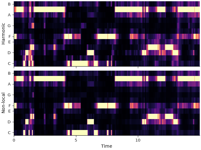
Local discontinuities and transients can be suppressed by using a horizontal median filter.

chroma_smooth = scipy.ndimage.median_filter(chroma_filter, size=(1, 9))


fig, ax = plt.subplots(nrows=2, sharex=True, sharey=True)
librosa.display.specshow(chroma_filter[idx], y_axis="chroma", x_axis="time", ax=ax[0])
ax[0].set(ylabel="Non-local")
ax[0].label_outer()

librosa.display.specshow(chroma_smooth[idx], y_axis="chroma", x_axis="time", ax=ax[1])
ax[1].set(ylabel="Median-filtered")

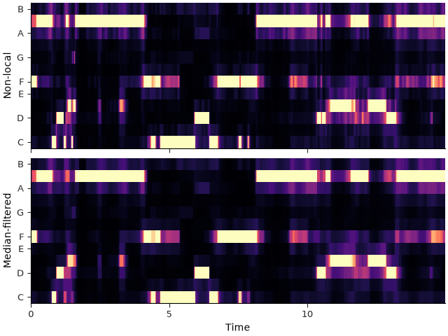
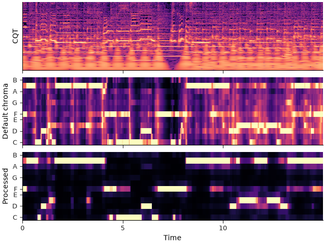
A final comparison between the CQT, original chromagram and the result of our filtering.

fig, ax = plt.subplots(nrows=3, sharex=True)
librosa.display.specshow(C[idx], vscale="dBFS",
                         y_axis="cqt_note", x_axis="time",
                         bins_per_octave=12*3, ax=ax[0])
ax[0].set(ylabel="CQT")
ax[0].label_outer()
librosa.display.specshow(chroma_orig[idx], y_axis="chroma", x_axis="time", ax=ax[1])
ax[1].set(ylabel="Default chroma")
ax[1].label_outer()
librosa.display.specshow(chroma_smooth[idx], y_axis="chroma", x_axis="time", ax=ax[2])
ax[2].set(ylabel="Processed")

Chroma variants

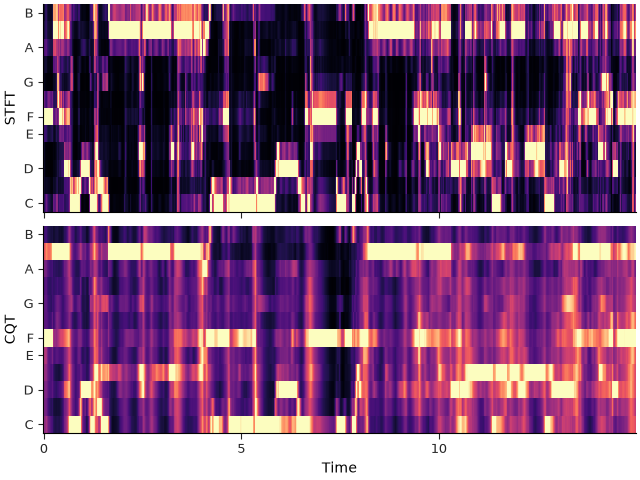
There are three chroma variants implemented in librosa: chroma_stft, chroma_cqt, and chroma_cens. chroma_stft and chroma_cqt are two alternative ways of plotting chroma. chroma_stft performs short-time fourier transform of an audio input and maps each STFT bin to chroma, while chroma_cqt uses constant-Q transform and maps each cq-bin to chroma.

A comparison between the STFT and the CQT methods for chromagram.

chromagram_stft = librosa.feature.chroma_stft(y=y, sr=sr)
chromagram_cqt = librosa.feature.chroma_cqt(y=y, sr=sr)


fig, ax = plt.subplots(nrows=2, sharex=True, sharey=True)
librosa.display.specshow(chromagram_stft[idx], y_axis="chroma", x_axis="time", ax=ax[0])
ax[0].set(ylabel="STFT")
ax[0].label_outer()

librosa.display.specshow(chromagram_cqt[idx], y_axis="chroma", x_axis="time", ax=ax[1])
ax[1].set(ylabel="CQT")

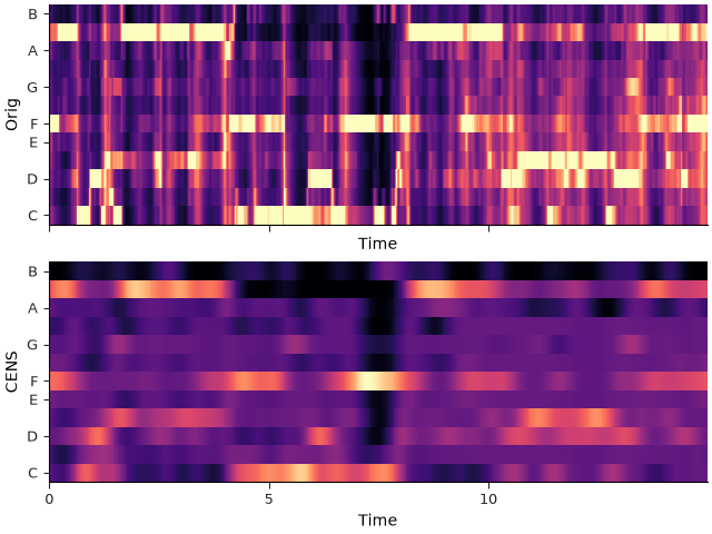
CENS features (chroma_cens) are variants of chroma features introduced in Müller and Ewart, 2011 [2], in which additional post processing steps are performed on the constant-Q chromagram to obtain features that are invariant to dynamics and timbre.

Thus, the CENS features are useful for applications, such as audio matching and retrieval.

Following steps are additional processing done on the chromagram, and are implemented in chroma_cens:

1. L1-Normalization across each chroma vector

2. Quantization of the amplitudes based on “log-like” amplitude thresholds

3. Smoothing with sliding window (optional parameter)

4. Downsampling (not implemented)

[2]

Meinard Müller & Sebastian Ewert. (2011). Chroma Toolbox: Matlab Implementations for Extracting Variants of Chroma-Based Audio Features. Proceedings of the 12th International Society for Music Information Retrieval Conference, 215–220. https://doi.org/10.5281/zenodo.1416032

A comparison between the original constant-Q chromagram and the CENS features.

chromagram_cens = librosa.feature.chroma_cens(y=y, sr=sr)


fig, ax = plt.subplots(nrows=2, sharex=True, sharey=True)
librosa.display.specshow(chromagram_cqt[idx], y_axis="chroma", x_axis="time", ax=ax[0])
ax[0].set(ylabel="Orig")

librosa.display.specshow(chromagram_cens[idx], y_axis="chroma", x_axis="time", ax=ax[1])
ax[1].set(ylabel="CENS")