Music Synchronization with Dynamic Time Warping

In this short tutorial, we demonstrate the use of dynamic time warping (DTW) for music synchronization which is implemented in librosa.

We assume that you are familiar with the algorithm and focus on the application. Further information about the algorithm can be found in the literature, e. g. [1].

Our example consists of two recordings of the same piece of music, where one is played at a different (and variable) tempo from the other. Our objective is now to find an alignment between these two recordings by using DTW.

# Code source: Stefan Balke
# License: ISC

import numpy as np
import matplotlib.pyplot as plt
from IPython.display import HTML

import librosa

Load Audio Recordings

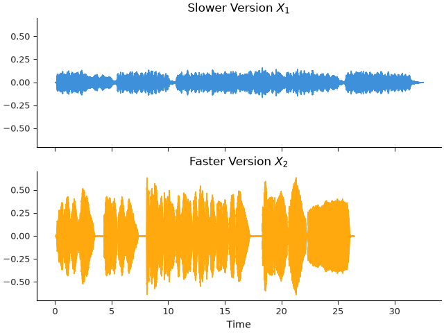
First, let’s load a first version of our audio recordings.

x_1, fs = librosa.loadx("drese")
# And a second version, with tempo variations
x_2, fs = librosa.loadx("drese2")

HTML(librosa.util.example_info("drese", html=True))

Jesu geh voran

By: Adam Drese (composer) | License: CC-BY-4.0

Source: https://www.audiolabs-erlangen.de/resources/MIR/2025-ChoraleBricks

Corpus: ChoraleBricks

Description

Excerpted from:
[1] Stefan Balke, Axel Berndt, and Meinard Müller.
ChoraleBricks: A Modular Multitrack Dataset for Wind Music Research
Transaction of the International Society for Music Information Retrieval (TISMIR), 8(1): 39–54, 2025.

Channels 1--3 include the Alto Sax, Clarinet and Trumpet recordings.

Channels 4 and 5 were synthesized independently by Brian McFee as follows:
- Channel 4 was recorded from a Roland SC-88 Pro with MIDI Piano
- Channel 5 was recorded from Vital using the "Synthetic Solo" (strings) preset

fig, ax = plt.subplots(nrows=2, sharex=True, sharey=True)
librosa.display.waveshow(x_1, sr=fs, ax=ax[0])
ax[0].set(title="Slower Version $X_1$")
ax[0].label_outer()

librosa.display.waveshow(x_2, sr=fs, ax=ax[1], color="C1")
ax[1].set(title="Faster Version $X_2$")

We can play them back using the IPython.display module.

from IPython.display import Audio

# Slower version (x_1):
Audio(x_1, rate=fs)

# Faster version (x_2):
Audio(x_2, rate=fs)

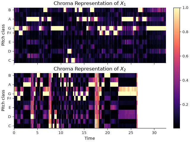
Extract Chroma Features

hop_length = 1024

x_1_chroma = librosa.feature.chroma_cqt(y=x_1, sr=fs,
                                         hop_length=hop_length)
x_2_chroma = librosa.feature.chroma_cqt(y=x_2, sr=fs,
                                         hop_length=hop_length)

fig, ax = plt.subplots(nrows=2, sharey=True, sharex=True)
img = librosa.display.specshow(x_1_chroma, x_axis="time",
                               y_axis="chroma", key="G:major",
                               hop_length=hop_length, ax=ax[0])
ax[0].label_outer()
ax[0].set(title="Chroma Representation of $X_1$", xlabel="")
librosa.display.specshow(x_2_chroma, x_axis="time",
                         y_axis="chroma", key="G:major",
                         hop_length=hop_length, ax=ax[1])
ax[1].set(title="Chroma Representation of $X_2$")
fig.colorbar(img, ax=ax)

Align Chroma Sequences

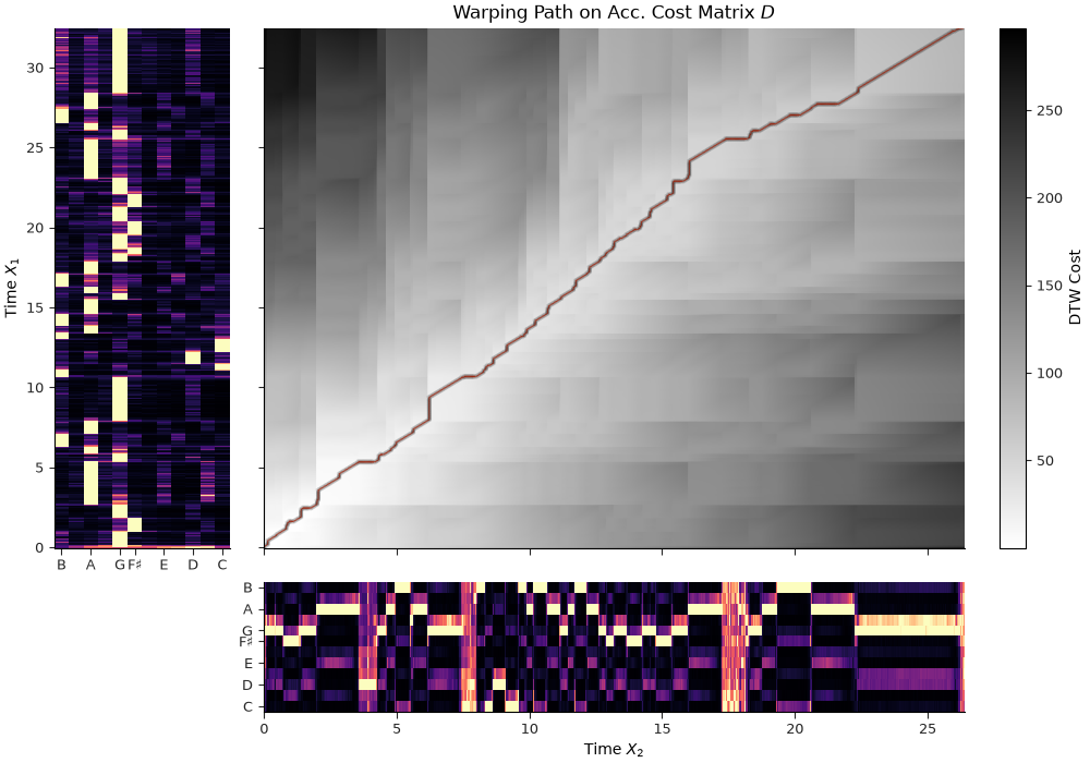
D, wp = librosa.sequence.dtw(X=x_1_chroma, Y=x_2_chroma, metric="cosine")
wp_s = librosa.frames_to_time(wp, sr=fs, hop_length=hop_length)

# By default, the path is returned in reverse order.  So let's put it forward
wp_s = wp_s[::-1]

# We'll make a subplot mosaic to show the chroma features for each signal
# aligned with the DTW cost matrix.
fig, ax = plt.subplot_mosaic(
        """
        ABB
        ABB
        .CC
        """, height_ratios=[2, 2, 1], width_ratios=[1, 2, 2], figsize=(10, 7))
librosa.display.specshow(x_1_chroma.T, y_axis="time", x_axis="chroma", key="G:major", sr=fs, hop_length=hop_length,
                         ax=ax["A"])
ax["A"].set(ylabel="Time $X_1$", xlabel="")
ax["A"].invert_xaxis() # Invert x-axis to match transposed chroma display
librosa.display.specshow(x_2_chroma, x_axis="time", y_axis="chroma", key="G:major", sr=fs, hop_length=hop_length,
                         ax=ax["C"])
ax["C"].set(xlabel="Time $X_2$", ylabel="")
img = librosa.display.specshow(D, x_axis="time", y_axis="time", sr=fs,
                               cmap="gray_r", hop_length=hop_length, ax=ax["B"])
ax["A"].sharey(ax["B"])
ax["C"].sharex(ax["B"])

# Plot the warping path as a quiver plot
dx, dy = np.diff(wp_s, axis=0, prepend=0).T
# Normalize the arrows to have unit length
norm = np.sqrt(dx**2 + dy**2) + librosa.util.tiny(dx)
dx /= norm
dy /= norm
q = ax["B"].quiver(wp_s[:, 1], wp_s[:, 0], dy, dx,
          angles="xy", pivot="tip", scale_units="xy", scale=10,
          color="C2", width=0.001, headwidth=20., headlength=20., headaxislength=10.)
librosa.display.highlight(artist=q, alpha=0.1)
ax["B"].set(title="Warping Path on Acc. Cost Matrix $D$")
fig.colorbar(img, ax=ax["B"], label="DTW Cost")

ax["B"].label_outer()

Alternative Visualization in the Time Domain

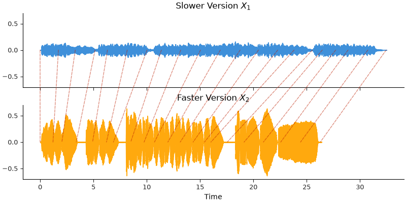
We can also visualize the warping path directly on our time domain signals. Red lines connect corresponding time positions in the input signals. (Thanks to F. Zalkow for the nice visualization.)

from matplotlib.patches import ConnectionPatch

fig, (ax_1, ax_2) = plt.subplots(nrows=2, sharex=True, sharey=True, figsize=(8,4))

# Plot x_2
librosa.display.waveshow(x_2, sr=fs, ax=ax_2, color="C1")
ax_2.set(title="Faster Version $X_2$")

# Plot x_1
librosa.display.waveshow(x_1, sr=fs, ax=ax_1)
ax_1.set(title="Slower Version $X_1$")
ax_1.label_outer()


n_arrows = 20
for tp1, tp2 in wp_s[::len(wp_s)//n_arrows]:
    # Create a connection patch between the aligned time points
    # in each subplot
    con = ConnectionPatch(xyA=(tp1, 0), xyB=(tp2, 0),
                          axesA=ax_1, axesB=ax_2,
                          coordsA="data", coordsB="data",
                          color="C2", linestyle="--",
                          alpha=0.5)
    con.set_in_layout(False)  # This is needed to preserve layout
    ax_2.add_artist(con)

Alignment and time stretching

We can now use the warping path to align the two signals. We will do this by applying a non-uniform time stretching to the slower signal $X_1$ so that it matches the faster signal $X_2$.

This requires two steps:

1. Convert the warping path to a timing grid

2. Use phase vocoding to stretch the slow signal

steps = librosa.sequence.path_to_steps(wp)

# Phase vocoding operates on the STFT of the signal
x_1_stft = librosa.stft(x_1, hop_length=hop_length)
# A bit of Griffin-Lim phase cleanup...

stft_stretched = librosa.phase_vocoder(x_1_stft, t_out=steps)
# Convert the stretched STFT back to the time domain
x_1_stretched = librosa.istft(stft_stretched, hop_length=hop_length, length=len(x_2))

We can now visualize and listen to the stretched signal in comparison to the faster signal.

fig, ax = plt.subplots(nrows=3, sharex=True, sharey=True)
librosa.display.waveshow(x_1, sr=fs, ax=ax[0])
librosa.display.waveshow(x_1_stretched, sr=fs, ax=ax[1])
librosa.display.waveshow(x_2, sr=fs, ax=ax[2], color="C1")
ax[0].label_outer()
ax[0].set(xlabel="", title="Slower $X_1$")
ax[1].label_outer()
ax[1].set(xlabel="", title="Stretched $X_1$")
ax[2].set(title="Faster $X_2$")

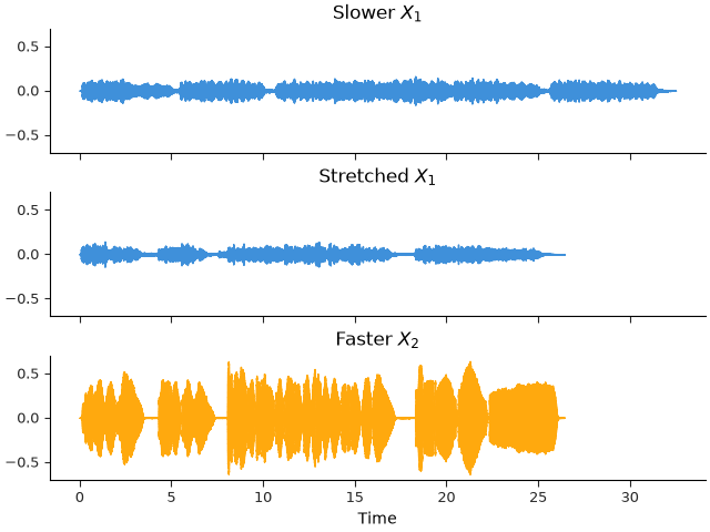
On playback, we can hear that there are some noticeable artifacts in the stretched signal, but it is time-aligned to the faster signal. Here we will play the original fast signal in the left channel and the time-stretched signal in the right channel.

🎧 This example is best experienced with headphones.

Audio(librosa.to_stereo(left=x_2, right=x_1_stretched), rate=fs)

We can also apply the time stretching in the opposite direction by setting the inverse parameter of path_to_steps to True.

steps_inv = librosa.sequence.path_to_steps(wp, inverse=True)
x_2_stft = librosa.stft(x_2, hop_length=hop_length)
stft2_stretched = librosa.phase_vocoder(x_2_stft, t_out=steps_inv)
x_2_stretched = librosa.istft(stft2_stretched, hop_length=hop_length, length=len(x_1))

And we can visualize the results just like before:

fig, ax = plt.subplots(nrows=3, sharex=True, sharey=True)
librosa.display.waveshow(x_1, sr=fs, ax=ax[0])
librosa.display.waveshow(x_2_stretched, sr=fs, ax=ax[1], color="C1")
librosa.display.waveshow(x_2, sr=fs, ax=ax[2], color="C1")
ax[0].label_outer()
ax[0].set(xlabel="", title="Slower $X_1$")
ax[1].label_outer()
ax[1].set(xlabel="", title="Stretched $X_2$")
ax[2].set(title="Faster $X_2$")

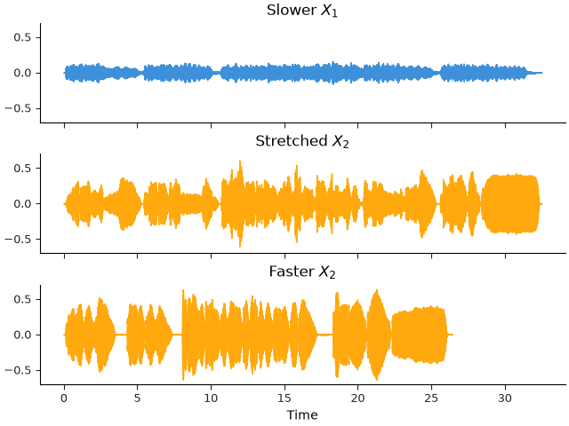
We will play the original slow signal in the left channel and the time-stretched signal in the right channel.

Audio(librosa.to_stereo(left=x_1, right=x_2_stretched), rate=fs)

Next steps…

Alright, you might ask where to go from here. Once we have the warping path between our two signals, we could realize different applications. One example is a player which enables you to navigate between different recordings of the same piece of music, e.g. one of Wagner’s symphonies played by an orchestra or in a piano-reduced version.

Literature

[1]

Meinard Müller, Fundamentals of Music Processing — Audio, Analysis, Algorithms, Applications. Springer Verlag, 2015.