

Note
Go to the end to download the full example code.
Laplacian segmentation#
This notebook implements the laplacian segmentation method of McFee and Ellis, 2014 [1], with a couple of minor stability improvements.
Throughout the example, we will refer to equations in the paper by number, so it will be helpful to read along.
# Code source: Brian McFee
# License: ISC
- Imports
numpy for basic functionality
scipy for graph Laplacian
matplotlib for visualization
sklearn.cluster for K-Means
IPython.display for metadata rendering
import numpy as np
import scipy
import matplotlib.pyplot as plt
from IPython.display import HTML

import sklearn.cluster

import librosa
First, we’ll load in a song
y, sr = librosa.loadx("fishin")
HTML(librosa.util.example_info("fishin", html=True))
Next, we’ll compute and plot a log-power CQT
BINS_PER_OCTAVE = 12 * 3
N_OCTAVES = 7
C = librosa.amplitude_to_db(np.abs(librosa.cqt(y=y, sr=sr,
                                        bins_per_octave=BINS_PER_OCTAVE,
                                        n_bins=N_OCTAVES * BINS_PER_OCTAVE)),
                            ref=np.max)

fig, ax = plt.subplots()
librosa.display.specshow(C, y_axis="cqt_hz", sr=sr,
                         bins_per_octave=BINS_PER_OCTAVE,
                         x_axis="time", ax=ax)
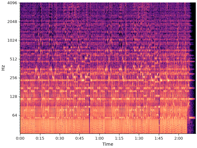
To reduce dimensionality, we’ll beat-synchronize the CQT
tempo, beats = librosa.beat.beat_track(y=y, sr=sr, trim=False)
Csync = librosa.util.sync(C, beats, aggregate=np.median)

# For plotting purposes, we'll need the timing of the beats
# we fix_frames to include non-beat frames 0 and C.shape[1] (final frame)
beat_times = librosa.frames_to_time(librosa.util.fix_frames(beats,
                                                            x_min=0),
                                    sr=sr)

fig, ax = plt.subplots()
librosa.display.specshow(Csync, bins_per_octave=BINS_PER_OCTAVE, sr=sr,
                         y_axis="cqt_hz", x_axis="time",
                         x_coords=beat_times, ax=ax)
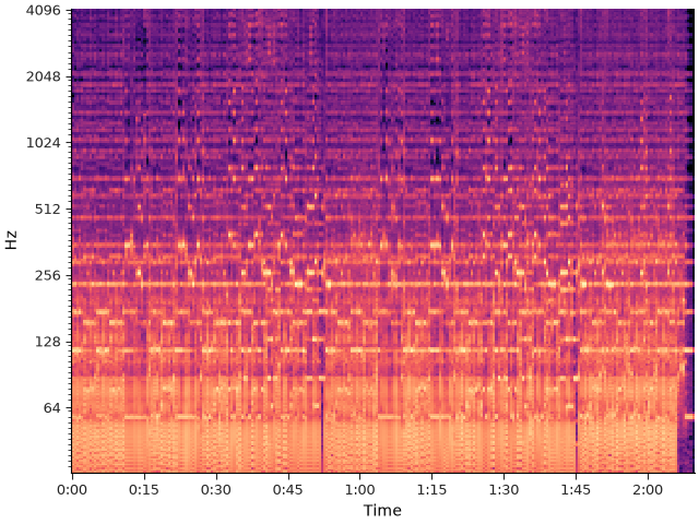
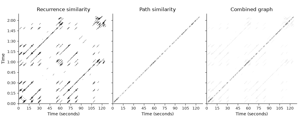
Let’s build a weighted recurrence matrix using beat-synchronous CQT (Equation 1) width=3 prevents links within the same bar mode=’affinity’ here implements S_rep (after Eq. 8)
We’ll also use some time-delay embedding to reduce false links.
Csync_stack = librosa.feature.stack_memory(Csync, n_steps=3, delay=1)
R = librosa.segment.recurrence_matrix(Csync_stack, width=3, mode="affinity",
                                      sym=True)

# Enhance diagonals with a median filter (Equation 2)
df = librosa.segment.timelag_filter(scipy.ndimage.median_filter)
Rf = df(R, size=(1, 7))
Now let’s build the sequence matrix (S_loc) using mfcc-similarity
\(R_\text{path}[i, i\pm 1] = \exp(-\|C_i - C_{i\pm 1}\|^2 / \sigma^2)\)
Here, we take \(\sigma\) to be the median distance between successive beats.
We’ll use librosa.feature.delta to compute the distance between successive beats.
mfcc = librosa.feature.mfcc(y=y, sr=sr)
Msync = librosa.util.sync(mfcc, beats)

path_distance = np.sum(librosa.feature.delta(Msync, axis=1)**2, axis=0)[1:]
sigma = np.median(path_distance)
path_sim = np.exp(-path_distance / sigma)

R_path = np.diag(path_sim, k=1) + np.diag(path_sim, k=-1)
And compute the balanced combination (Equations 6, 7, 9)
Plot the resulting graphs (Figure 1, left and center)
fig, ax = plt.subplots(ncols=3, sharex=True, sharey=True, figsize=(10, 4))
librosa.display.multiplot("specshow", Rf, R_path, A,
                          titles=["Recurrence similarity", "Path similarity", "Combined graph"],
                          cmap="gray_r",
                          y_axis="time", x_axis="s",
                          y_coords=beat_times, x_coords=beat_times,
                          axes=ax)
Now let’s compute the normalized Laplacian (Eq. 10)
L = scipy.sparse.csgraph.laplacian(A, normed=True)


# and its spectral decomposition
evals, evecs = scipy.linalg.eigh(L)


# We can clean this up further with a median filter.
# This can help smooth over small discontinuities
evecs = scipy.ndimage.median_filter(evecs, size=(9, 1))


# cumulative normalization is needed for symmetric normalize laplacian eigenvectors
Cnorm = np.cumsum(evecs**2, axis=1)**0.5

# If we want k clusters, use the first k normalized eigenvectors.
# Fun exercise: see how the segmentation changes as you vary k

k = 5

X = evecs[:, :k] / Cnorm[:, k-1:k]
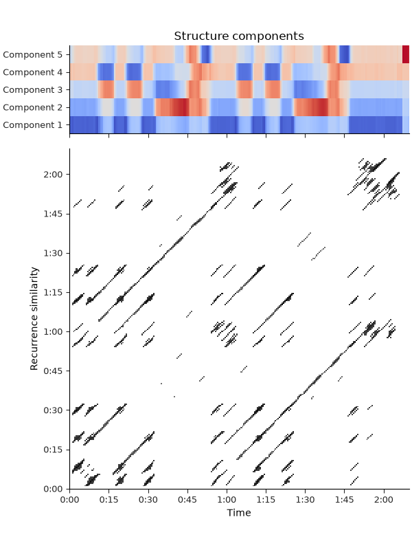
We can now plot the resulting representation along with the recurrence matrix to see how the structural components align with repeating patterns.
Each structural component is an normalized eigenvector with dimension equal to the number of beats. The collection of structural components can be used as features to describe each beat, which can then be clustered to identify segments.
fig, ax = plt.subplots(nrows=2, sharex=True, figsize=(6, 8),
                       layout="compressed",
                       gridspec_kw={"height_ratios": [1, 4]})
librosa.display.specshow(Rf, cmap="gray_r", y_axis="time", x_axis="time",
                         y_coords=beat_times, x_coords=beat_times, ax=ax[1])
ax[1].set(ylabel="Recurrence similarity")

librosa.display.specshow(X.T,
                         x_axis="time",
                         x_coords=beat_times, ax=ax[0])
ax[0].set(yticks=np.arange(k), yticklabels=[f"Component {i+1}" for i in range(k)])
ax[0].set(title="Structure components")
ax[0].label_outer()
Let’s use these k components to cluster beats into segments (Algorithm 1)
KM = sklearn.cluster.KMeans(n_clusters=k, n_init="auto", random_state=0)

seg_ids = KM.fit_predict(X)
Now that we have the segment id for each beat, we can identify the boundaries by where the segment id changes.
bound_beats = 1 + np.flatnonzero(seg_ids[:-1] != seg_ids[1:])

# Count beat 0 as a boundary
bound_beats = librosa.util.fix_frames(bound_beats, x_min=0)

# Compute the segment label for each boundary
bound_segs = list(seg_ids[bound_beats])

# Convert beat indices to frames
bound_frames = beats[bound_beats]

# Make sure we cover to the end of the track
bound_frames = librosa.util.fix_frames(bound_frames,
                                       x_min=None,
                                       x_max=C.shape[1]-1)
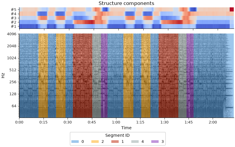
And plot the final segmentation alongside the CQT and the structure components. We can use mir_eval’s annotation display to generate the patches for us. We’ll draw the spectrogram in grayscale so that the color-coding for each section is clearly visible.
import itertools
import mir_eval.display

bound_times = librosa.frames_to_time(bound_frames)
freqs = librosa.cqt_frequencies(n_bins=C.shape[0],
                                fmin=librosa.note_to_hz("C1"),
                                bins_per_octave=BINS_PER_OCTAVE)

fig, ax = plt.subplots(figsize=(8, 5), nrows=2, gridspec_kw={"height_ratios": [1, 4]},
                       layout="compressed")
librosa.display.specshow(X.T, x_axis="time", x_coords=beat_times, ax=ax[0])
ax[0].set(yticks=np.arange(k), yticklabels=[f"#{i+1}" for i in range(k)])
ax[0].set(title="Structure components")
ax[0].label_outer()
librosa.display.specshow(C, y_axis="cqt_hz", sr=sr,
                         bins_per_octave=BINS_PER_OCTAVE,
                         cmap="gray_r",
                         x_axis="time", ax=ax[1])

# Convert boundary times to a set of intervals
intervals = np.asarray(list(itertools.pairwise(bound_times)))
mir_eval.display.segments(intervals, bound_segs, ax=ax[1], alpha=0.5)
fig.legend(loc="outside lower center", title="Segment ID", ncols=k)
Summary#
In the final plot above, we can see that each colored region corresponds to a distinct pattern that repeats throughout the song. It should be clear that the segmentation boundaries (changes in color over time) correspond to changes in the structural components (top panel). Note that the segment id values (0, 1, 2, …) correspond to K-Means cluster identifiers, and are essentially arbitrary with no relationship to the temporal order in which segments actually occur. Still, the pattern of repetition and grouping of regions is clear and can be used to quickly understand the structure of the song.
Total running time of the script: (0 minutes 5.097 seconds)