

Note
Go to the end to download the full example code.
Harmony and chroma#
This section introduces tools for analyzing harmonic content of audio recordings.
Frequencies and harmonics#
In the previous section, we saw how to identify the fundamental frequency (f0) of a monophonic signal. This is the frequency that we usually identify as the “pitch” of a sound. However, sound is often much more complex than just a single frequency. Most interesting sounds contain energy and many related frequencies, and in the case of musical instruments (including human voice), these are often identified by the harmonics of the fundamental frequency. For a frequency f, the n-th harmonic (for n = 1, 2, 3, …) is the frequency n*f.
import librosa
import numpy as np
import matplotlib.pyplot as plt
from IPython.display import HTML

y, sr = librosa.loadx("trumpet")
HTML(librosa.util.example_info("trumpet", html=True))
S = np.abs(librosa.stft(y))
fig, ax = plt.subplots()
img = librosa.display.specshow(S, vscale="dBFS",
                               x_axis="time", y_axis="log", ax=ax)
librosa.display.colorbar_db(img, label="dBFS")
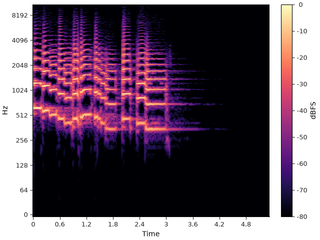
In the trumpet example above, we can observe a repeating vertical pattern. If there is energy (bright color) at f0 (e.g., around 620 Hz at the beginning of the signal), there is also energy at twice that frequency (~1240 Hz), three times that frequency (1860 Hz), and so on. This distribution of energy across the harmonics of the fundamental contributes to the timbre of the instrument.
Constant-Q spectrum#
So far, we’ve relied on the Short-time Fourier Transform (STFT) to analyze the frequency content of a signal as it changes over time. The STFT has a couple of limitations for harmonic content analysis:
The set of frequencies is spaced linearly between 0 and sr/2. This is not wrong per se, but it does not directly align with notions of harmonics, which are spaced geometrically.
The frame length is fixed for all frequencies (n_fft). This means that low frequencies will complete a small number of cycles within the frame, while high frequencies will complete many cycles. This results in relatively poor discrimination of low frequencies, which can be important when analyzing musical signals.
The constant-Q transform (CQT) was developed to circumvent these issues. The underlying idea is quite similar to the STFT, in that the signal is chopped into small pieces and compared to a set of reference sinusoids at a fixed set of frequencies. The differences are that 1) the frequencies are chosen to be geometrically spaced, so that the n`th frequency is given as `2**(n / bins_per_octave) * f_min (for a minimum analysis frequency f_min > 0), and 2) rather than fixing the duration of the frame across frequencies, the CQT fixes the number of cycles completed across frequencies, and allows the frame length to vary (while remaining centered at a given index).
Computing the CQT of a signal in librosa can be done by the following code:
By default, the CQT uses 12 bins per octave, starting at a minimum frequency of C1 (about 32.7 Hz), and spanning 7 octaves to cover the range 32.7 (C1) to 3951 (B7).
We can visualize a CQT in much the same way as an STFT through the specshow function, but note that the y_axis parameter is now different:
fig, ax = plt.subplots()
img = librosa.display.specshow(C, vscale="dBFS",
                               x_axis="time", y_axis="cqt_hz",
                               ax=ax)
librosa.display.colorbar_db(img, label="dBFS")
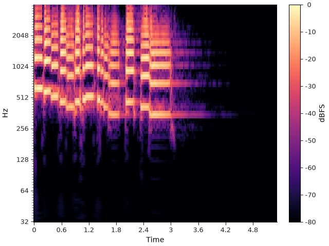
The image above should look somewhat similar to the visualization of the STFT, with two exceptions:
The frequency resolution is lower: we have only 84 frequencies now instead of 1025.
The frequency range is lower: the plot stops at about 4 KHz instead of 11 KHz in the STFT.
Both of these can be adjusted by setting parameters in the CQT. For example, to use more bins per octave than the default 12, we can set bins_per_octave=36. Any positive integer is supported here, though typically odd multiples of twelve are appropriate for increasing resolution while retaining alignment to the 12TET / A440 system.
Note that when you increase the number of bins per octave, you must also increase the number of bins accordingly. So if we go from 12 to 36 bins per octave, we should also go from 84 to 252 bins to retain the same frequency range. You can expand or contract the frequency range simply by changing the n_bins parameter.
Let’s create a new CQT, with a higher frequency resolution and a slightly higher frequency range.
We can also visualize like before, but we will need to tell specshow to use the correct number of bins per octave. (See Frequency ranges for more information on configuring frequency ranges in specshow.)
fig, ax = plt.subplots()
img = librosa.display.specshow(C, vscale="dBFS",
                               x_axis="time", y_axis="cqt_hz",
                               bins_per_octave=12 * 3,
                               ax=ax)
librosa.display.colorbar_db(img, label="dBFS")
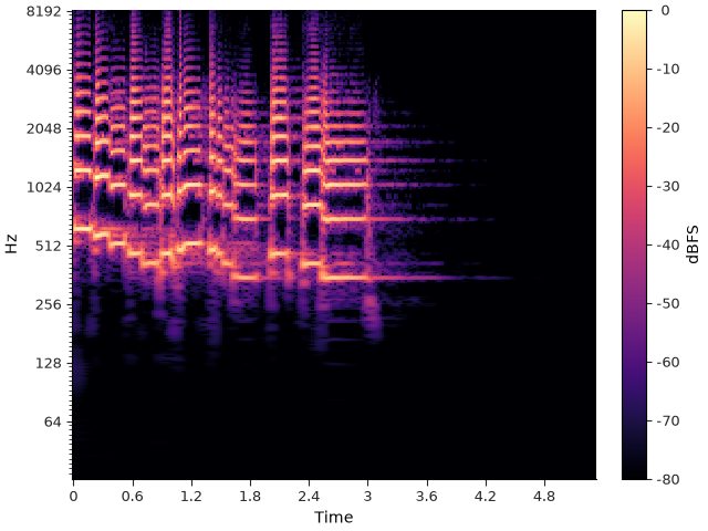
Visually, the CQT plot should now look very similar to the STFT plot we started with. However, these are numerically quite different objects:
STFT shape=(1025, 230)
CQT shape=(288, 230)
Aside from being a smaller representation, the CQT turns out to be a more convenient object to work with than the STFT for extracting harmonically related frequency content.
A more complex example#
The trumpet example above is monophonic: there is only one sound source, and at most one note sounding at any given time (though there will be energy at multiple frequencies for each note).
Let’s now look at a slightly more complex example, now involving multiple instruments and simultaneous notes.
from IPython.display import Audio

y, sr = librosa.loadx("sweetwaltz", duration=15)
HTML(librosa.util.example_info("sweetwaltz", html=True))
Audio(url=librosa.example("sweetwaltz", url=True))
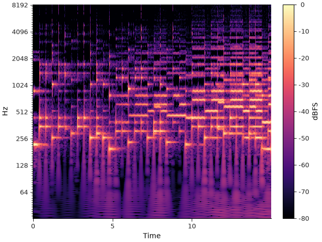
As before, we can compute and visualize the CQT of this example.
C = librosa.cqt(y=y, sr=sr,
                bins_per_octave=12*3,
                n_bins=12*3*8)

fig, ax = plt.subplots()
img = librosa.display.specshow(C, vscale="dBFS",
                               x_axis="time",
                               y_axis="cqt_hz",
                               bins_per_octave=12*3,
                               ax=ax)
librosa.display.colorbar_db(img, label="dBFS")
Chroma#
At this point, it becomes much more difficult to distinguish notes (fundamental frequencies) from harmonics, and generally there is much more information to make sense of.
Often when we analyze the harmonic content of a recording, we are less interested in exact frequencies and pitches than we are in pitch classes, i.e., pitch reduced to a single octave. This is what chroma representations are meant to capture, and they generally work by aggregating information from a time-frequency representation (in our case, a CQT) at all frequencies corresponding to each pitch class. For example, the C pitch class would collect energy from frequencies 32.7, 65.4, 130.8, 261.6, etc. The C♯ pitch class would collect energy from 34.6, 69.3, 138.6, 277.2, etc., and this pattern repeats for all pitch classes from C to B.
Librosa implements a few methods for constructing chroma representations, but here we will demonstrate the CQT-based method. By default, this will use a 36-bin-per-octave CQT spanning 7 octaves.
sphinx_gallery_thumbnail_number = 5 We can visualize this with specshow as well, now setting the y_axis mode to chroma. We’ll plot this underneath the CQT plot from above so the two can be directly compared.
fig, ax = plt.subplots(nrows=2, sharex=True, height_ratios=(3, 1))
imgcqt = librosa.display.specshow(C, vscale="dBFS",
                                  x_axis="time",
                                  y_axis="cqt_hz",
                                  bins_per_octave=12*3,
                                  ax=ax[0])
librosa.display.colorbar_db(imgcqt, label="dBFS")
ax[0].label_outer()  # only show x-axis labels on the bottom plot
imgchroma = librosa.display.specshow(chroma,
                                     x_axis="time",
                                     y_axis="chroma",
                                     ax=ax[1])
fig.colorbar(imgchroma, ax=ax[1], aspect=20/3)  # aspect compensates for the 3:1 height ratio of these plots
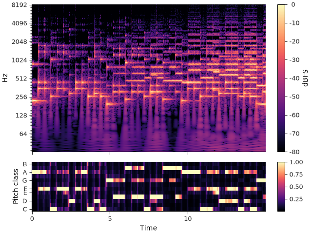
Each row of the chroma corresponds to a pitch class, and the value corresponds to the amount of relative energy detected within that pitch class. Note that the values are now normalized to the range [0, 1], which is intended to provide some robustness to changes in loudness.
Unlike f0 estimation, multiple pitch classes may be active at any given time.
Chroma features are therefore often used as a feature representation for automatic chord
estimation, where each time step is mapped to a chord label such as F:maj or D:min.
While it is possible to build a basic chord estimation method using template matching
(see the example in librosa.sequence.viterbi_discriminative), modern methods generally
involve supervised machine learning, and are out of scope for librosa.
Summary#
This section introduced the constant-Q transform and chroma representations as a way of representing harmonic content in musical signals. The methods described above are quite basic, however, and there are numerous ways to improve upon them with more advanced pre- and post-processing techniques. If you want to learn more about designing effective chroma representations, you may want to look at Enhanced chroma.
Total running time of the script: (0 minutes 3.202 seconds)