

Note
Go to the end to download the full example code.
Annotations and mir_eval integration#
This section illustrates integration of librosa display with the mir_eval library’s utilities
for visualizing annotations.
Librosa’s display module broadly covers the visualization of signals and features derived
from signals. It generally does not support visualizing annotations of signals,
such as estimated event timings (onsets or beats), pitch trajectories, or labeled intervals.
In some of the earlier sections of this tutorial, we have seen how to plot these kinds of
annotations using matplotlib directly. However, the mir_eval library provides a set of
utilities for visualizing annotations in a more direct and convenient way.
In this final section of the display tutorial, we’ll show how to use both
of these packages together to visualize annotations alongside signal content.
mir_eval.display#
The mir_eval.display module provides a variety of functions for visualizing many kinds
of annotations. Here we’ll focus on three kinds: pitch contours, event timings, and labeled
intervals.
Because both mir_eval and librosa are built on top of matplotlib, they can be used
together seamlessly.
Pitch contours#
First, we can replicate the earlier example of estimating the fundamental
frequency of a trumpet recording.
We previously used matplotlib’s plot function for this, but mir_eval.display can do a
bit more for us.
For example, the pyin f0 estimator by default will leave unvoiced regions as np.nan.
We can also ask pyin to fill in a best guess by using fill_na=None, and indicate
unvoiced regions by a negative value.
mir_eval will detect this and shade the unvoiced regions in the plot.
import numpy as np
import matplotlib.pyplot as plt
from IPython.display import HTML
import librosa
import mir_eval.display

y, sr = librosa.loadx("trumpet")
HTML(librosa.util.example_info("trumpet", html=True))
Estimate the f0 using pyin
f0, voiced_flag, voiced_probs = librosa.pyin(y, fmin=librosa.note_to_hz("C2"),
                                             fmax=librosa.note_to_hz("C7"),
                                             fill_na=None,
                                             sr=sr)
# Mark unvoiced frames as negative.
# Everywhere that `voiced_flag[i]` is False, we will multiply `f0[i]` by -1.
f0_voiced_unvoiced = f0 * (-1) ** (~voiced_flag)
Visualize the spectrogram using specshow and overlay f0 using mir_eval.display.pitch
fig, ax = plt.subplots()
stft = librosa.stft(y)
librosa.display.specshow(stft, vscale="dBFS", x_axis="time", y_axis="log_oct3", ax=ax)
hl = librosa.display.highlight(ax=ax, linewidth=6)

# Get the time values for f0
times = librosa.times_like(f0, sr=sr)
mir_eval.display.pitch(times, f0_voiced_unvoiced,
                       ax=ax,
                       unvoiced=True,
                       label="pyin f0 estimate",
                       color="C2",
                       linewidth=3,
                       path_effects=hl)
ax.legend(loc="upper right")
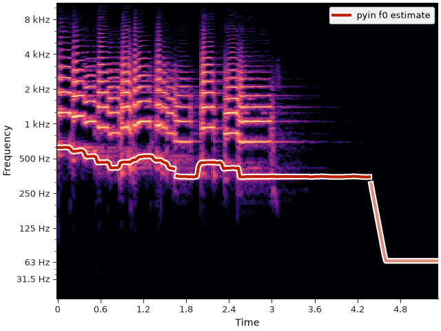
In the plot above, we can now clearly see the that the detected unvoiced region at the end of the signal (from times 4.3 to 5.0 seconds) is drawn in a lighter color. Visualizing unvoiced regions in this way can be helpful for understanding the behavior of f0 estimation on certain examples, in particular when it makes voicing estimation errors.
Event timings#
Event timings are another common type of annotation, and mir_eval.display provides a
convenient function for visualizing them as vertical lines.
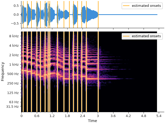
Here, we’ll use the onset detection function from librosa to detect the onsets
of the trumpet signal, and then visualize them using mir_eval.display.events.
This can be overlaid on any plot with a horizontal time axis, such as a waveform or
spectrogram. Here we’ll show both.
onsets = librosa.onset.onset_detect(y=y, sr=sr, units="time")

fig, ax = plt.subplots(nrows=2, sharex=True, gridspec_kw={"height_ratios": [1, 3]})
librosa.display.waveshow(y, sr=sr, ax=ax[0])
mir_eval.display.events(onsets, ax=ax[0], color="C1", label="estimated onsets")
ax[0].legend(loc="upper right")
ax[0].label_outer()
librosa.display.specshow(stft, vscale="dBFS", x_axis="time", y_axis="log_oct3", ax=ax[1])
hl = librosa.display.highlight(ax=ax[1], linewidth=3)
mir_eval.display.events(onsets, ax=ax[1], color="C1", label="estimated onsets",
                        path_effects=hl)
ax[1].legend(loc="upper right")
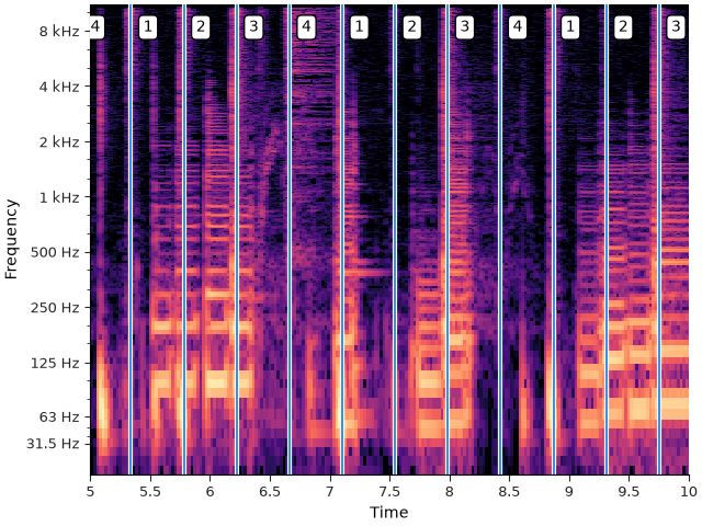
Events can also be labeled with text, which can be useful for visualizing beat events with
metrical position.
For this example, we’ll use a longer musical excerpt and detect beats using
librosa.beat.beat_track.
y, sr = librosa.loadx("choice")
HTML(librosa.util.example_info("choice", html=True))
Detect beats and visualize them with mir_eval.display.events
tempo, beats = librosa.beat.beat_track(y=y, sr=sr, units="time", trim=False)
# A quick hack to label the beats as 1, 2, 3, 4, ...
# In reality, you would want to use a downbeat estimator here, but this
# hack suffices for demonstration purposes.
beat_labels = [f"{(i % 4) + 1}" for i in range(len(beats))]

fig, ax = plt.subplots()
stft = librosa.stft(y)
librosa.display.specshow(stft, vscale="dBFS", x_axis="time", y_axis="log_oct3", ax=ax)
hl = librosa.display.highlight(ax=ax, linewidth=3)
mir_eval.display.events(beats, ax=ax, path_effects=hl,
                        labels=beat_labels)
# Zoom in to see labels more clearly
ax.set(xlim=[5, 10])
Labeled intervals#
Probably the most common type of annotation in audio data is a collection of labeled time intervals.
y, sr = librosa.loadx("trumpet")
stft = librosa.stft(y)

# Estimate f0
f0, voiced_flag, voiced_probs = librosa.pyin(y, fmin=librosa.note_to_hz("C2"),
                                             fmax=librosa.note_to_hz("C7"),
                                             sr=sr)

# Quantize to integer MIDI numbers
f0_midi = np.round(librosa.hz_to_midi(f0))

# Find the frame indices where f0_midi changes value
boundaries = np.where(np.diff(f0_midi) != 0)[0] + 1

# Convert boundaries to start/end intervals
intervals = np.column_stack([np.concatenate([[0], boundaries]),
                             np.concatenate([boundaries, [len(f0_midi)]])])

# Convert the MIDI numbers to note names, using F dorian as the key
# Unvoiced (nan) frames will be labeled with an empty string
notes = librosa.midi_to_note(f0_midi[intervals[:, 0]], key="F:dorian")

fig, ax = plt.subplots(figsize=(10, 4))
# Plot the spectrogram in grayscale so we can overlay colors
librosa.display.specshow(stft, vscale="dBFS",
                         x_axis="time", y_axis="fft_note", ax=ax,
                         cmap="gray_r")

# Label the intervals with the detected notes
mir_eval.display.segments(librosa.frames_to_time(intervals, sr=sr),
                          notes,
                          ax=ax, text=True, alpha=0.5)
ax.set(xlim=[0, 4.5])
fig.legend(loc="outside center right")
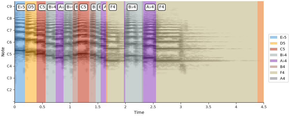
In the plot above, each segment is labeled according to the detected note within the
time interval, and mir_eval.display.segments automatically colors each segment according to
the note name.
While we have used pitch detection to generate the intervals and labels here,
any kind of labeled segmentation can be visualized in this way.
The segmentation example shows similar usage in the
context of structural analysis.
Summary#
Librosa and mir_eval can be used together to visualize annotations and signal content
together.
The examples above illustrate only the simplest and most common uses, but there are many more
things that you can do with mir_eval.display, including visualizing multiple f0 estimates,
piano roll displays, or comparison of different annotations.
Here we have focused on just the functionality that most clearly integrates with waveform or
spectrogram displays.
Total running time of the script: (0 minutes 2.587 seconds)