librosa.feature.inverse.mel_to_stft

librosa.feature.inverse.mel_to_stft(M, *, sr=22050, n_fft=2048, power=2.0, **kwargs)

Approximate STFT magnitude from a Mel power spectrogram.

Parameters:

Mnp.ndarray [shape=(…, n_mels, n), non-negative]

The spectrogram as produced by feature.melspectrogram

srnumber > 0 [scalar]

sampling rate of the underlying signal

n_fftint > 0 [scalar]

length of the FFT frame of the resulting STFT; the output has 1 + n_fft // 2 frequency bins

powerfloat > 0 [scalar]

Exponent for the magnitude melspectrogram

**kwargs

additional keyword arguments for Mel filter bank parameters

fminfloat >= 0 [scalar]

lowest frequency (in Hz)

fmaxfloat >= 0 [scalar]

highest frequency (in Hz). If None, use fmax = sr / 2.0

htkbool [scalar]

use HTK formula instead of Slaney

norm{None, ‘slaney’, or number} [scalar]

If ‘slaney’, divide the triangular mel weights by the width of the mel band (area normalization). If numeric, use librosa.util.normalize to normalize each filter by to unit l_p norm. See librosa.util.normalize for a full description of supported norm values (including +-np.inf). Otherwise, leave all the triangles aiming for a peak value of 1.0

dtypenp.dtype

The data type of the output basis. By default, uses 32-bit (single-precision) floating point.

Returns:

Snp.ndarray [shape=(…, 1 + n_fft // 2, t), non-negative]

An approximate linear magnitude spectrogram

See also

librosa.feature.melspectrogram

librosa.stft

librosa.filters.mel

librosa.util.nnls

Examples

>>> y, sr = librosa.loadx('trumpet')
>>> S = librosa.util.abs2(librosa.stft(y))
>>> mel_spec = librosa.feature.melspectrogram(S=S, sr=sr)
>>> S_inv = librosa.feature.inverse.mel_to_stft(mel_spec, sr=sr)

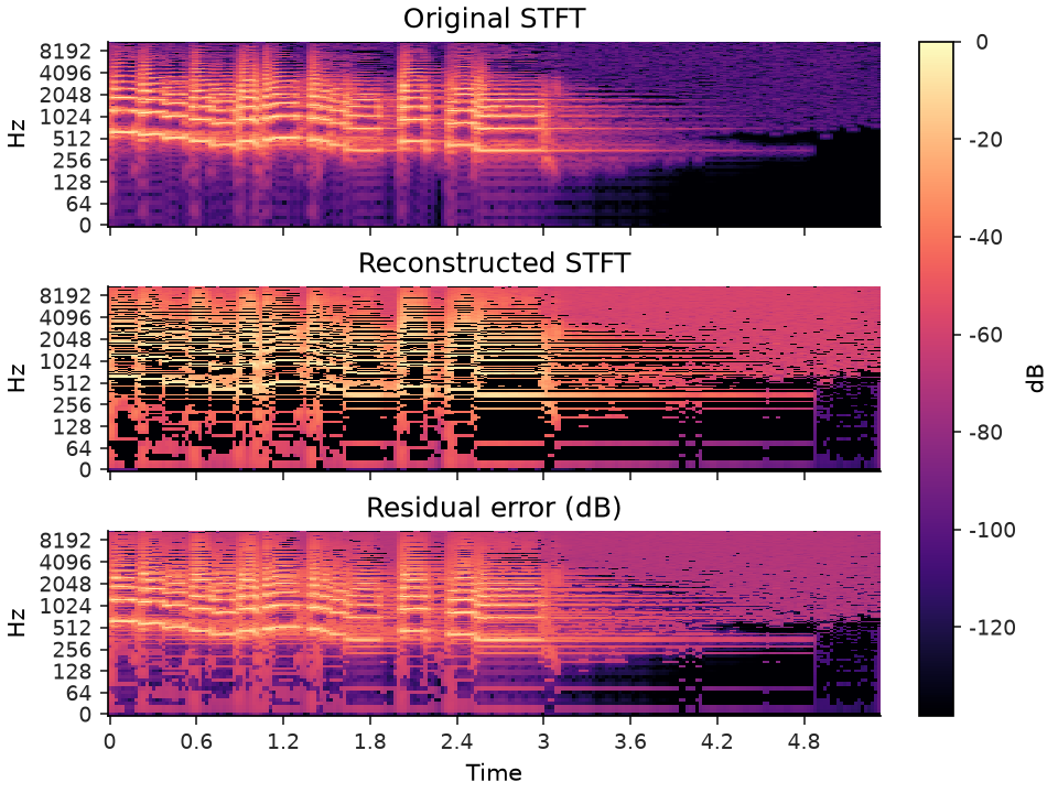
Compare the results visually

>>> import matplotlib.pyplot as plt
>>> fig, ax = plt.subplots(nrows=3, sharex=True, sharey=True)
>>> img = librosa.display.specshow(S, vscale='dBFS[power]', top_db=None,
...                          y_axis='log', x_axis='time', ax=ax[0])
>>> ax[0].set(title='Original STFT')
>>> ax[0].label_outer()
>>> librosa.display.specshow(S_inv, vscale='dBFS[power]', top_db=None,
...                          y_axis='log', x_axis='time', ax=ax[1])
>>> ax[1].set(title='Reconstructed STFT')
>>> ax[1].label_outer()
>>> librosa.display.specshow(S_inv - S, vscale=f'dB[power,{S.max()}]', top_db=None,
...                          vmax=0, y_axis='log', x_axis='time', ax=ax[2])
>>> ax[2].set(title='Residual error (dB)')
>>> librosa.display.colorbar_db(img, ax=ax)